


 nueva página del texto (beta)
 Inglés (pdf)
 Artículo en XML
 Referencias del artículo
 Enviar artículo por email
 Citado por SciELO
  Similares en
SciELO
Similares en
SciELO 
 Permalink
1. Introduction
According to the Food and Agriculture Organization of the United Nations (FAO), while fish farming has been expanding steadily world-wide in the years, unsustainable fishing declined or stabilized (Food and Agriculture Organization, 2020). Considering that water scarcity is intensifying, this growing demand for fish is making fish farmers look for production methods that allow them to produce more in increasingly smaller areas, using as little water as possible. In practice, which means the water is kept in the ponds as long as possible, reducing its recirculation. As a result, organic and inorganic particles such as silt, sediment, sand, and algae accumulate in the ponds, thus making the water cloudy.
Particles are defined as suspended when they are larger than 2 microns or dissolved otherwise. Usually, there is a myriad of suspended particles in the pounds, but it is the clay and other minerals that, along with the biomass from algae, impact the water transparency the most (Brezonik et al., 2019). They occur naturally due to the erosion caused by storms or the emergence of organic matter in the ponds and, by themselves, they are not harmful. The problem is that these particles absorb or reflect light, so that a large quantity of them may effectively gloom the water, thus increasing its turbidity. Briefly, turbidity is directly proportional to the amount of solids suspended in water, and inversely proportional to its transparency (Rügner et al., 2013).
Several studies show that the levels of water turbidity influence aquaculture. For example, Lowe et al. (2015) conducted an experiment in which five groups of fish were farmed under different turbidity levels to determine whether their food-seeking and consumption abilities would be affected by turbidity. The researchers reported that the fishes subjected to turbidity levels equal or greater than 40 NTU1 had a significant weight loss compared to the others, a result that is corroborated by Huenemann et al. (2012) and many others.
On the other hand, Chapman et al. (2014) reveals that a higher water transparency has a negative impact on feeding behavior and species diversity, besides compromising fish embryos development. Similar remarks are made in Hasenbein et al. (2013), who noted that the clearer the water, the lower the feed consumption. This evidence suggests that the transparency of the water bodies must be constantly monitored to allow the farmers to determine the proper amount of feed that must be provided at a given time for the fishes.
Transparency also has an indirect impact on fish. By partially blocking the passage of light, turbid waters prevent the formation of algae that, besides complementing the nourishment of fishes, help to keep the oxygenation of the pounds during the day through photosynthesis. However, transparent waters make those algae develop excessively and, since they also consume oxygen, which could bring the oxygenation of the pounds to critical levels in low light periods (Bhatnagar & Devi, 2013; Domingues et al., 2011).
The best-known method to measure the transparency of water is the Secchi disc created by Pietro Ângelo Secchi in 1865, which shows how deep the sun’s rays can traverse a given water body. To do that, a plain disc painted with alternating black and white quadrants is attached to a pole or string and progressively lowered into a water body until the observer can no longer see it. The depth at which this happens gives a measure of the transparency of the water based not only on its color but also on its spectral response to the light.
Many farmers use the Secchi disk because it is a simple and low-cost technique. However, it is a manual and inefficient procedure that requires a person to inspect each pond and measure the transparency data. There are also devices known as turbidimeters that can make the process easier. A turbidimeter determines how much the suspended particles of a water body absorb or refract the intensity of the light (Parra, 2018), yielding an estimated value for the water transparency shown in a digital display.
Although quite sophisticated when compared to the Secchi method, most turbidimeters still require manual data gathering, that is, farmers need to measure the water transparency pond by pond, so in practice they are not much better than the disks. Some models can be installed permanently within the ponds to last gather measures automatically and transmit them over long distances wirelessly, which is certainly practical because it does not require an operator to move from pond to pond to gather data. However, each pond must have its own turbidimeter, which may render the solution too costly.
Remote sensing techniques can also be used to measure water transparency by using, for example, multispectral images. In this approach, the reflectance levels of the water to the solar radiation are analyzed at different wavelengths, which gives a quite accurate transparency measure. Lim and Choi (2015) investigated the spectral responses of the Landsat 8 satellite in the Nakdong River in South Korea, and their results showed that the reflectance of bands 2 to 5 was indeed correlated with the water transparency. Huovinen et al. (2019) also reported related results.
Unfortunately, the trajectory of the satellites and the resolution of their images prevent them from being used for fish farming efficiently, so that this approach is restricted to substantial portions of water, such as oceans or large lakes. Images captured by remotely piloted aircraft (RPA) are more efficient to analyze smaller water bodies because they can get closer to the ponds. The aircraft can also carry different equipment and devices to the field, making them a better solution for remote sensing in fish farming environments.
Problems commonly faced when capturing images of water bodies via RPAs are light reflections caused by the relative position of the sun and waves caused by the wind, which can yield visual distortions that may compromise the analysis. Those issues can be mitigated through a proper choice of the spectral band for a given analysis, and careful pre-processing of the images.
In this work, we describe a prototype that estimates the levels of transparency of fishponds through the pictures taken with special cameras embedded in an RPA that flies over the area of interest. This solution has been validated in the field, at a fish farm in Toledo city, state of Paraná - Brazil, and the estimations obtained this way were consistent with the results got via traditional measurement methods.
2. Materials and methods
2.1. Prototype development
A Secchi disk is a disk that is painted in alternating black and white quadrants and has a diameter between 25 and 45 centimeters, a size that favors its handling and prevent many reading errors due light reflection on water surface. The disk is attached to a rope marked at appropriate intervals with waterproof markings and is lowered into a water body until the observer can no longer see it. This depth of disappearance, called the Secchi depth, is a measure of the transparency of the water.
Mutatis mutandis, the working principles of the Secchi disks are the same employed in this project, with the disk being replaced by a conic target 40 cm high and diameter ranging from 0 to 93 cm, which was built with a 0.5 mm galvanized steel sheet. This cone was painted with black and white stripes 4 centimeters wide, amounting to 5 black stripes and 5 white. When seen from the above, the cone seems like a target where its tip is the bull's eye. When immersed in a water body, the shape of that “target” allows an observer to infer the turbidity by counting many stripes that are visible: the more transparent the water, the more stripes will be reflecting the solar radiation. The cone can also be detected by a capture device (an RPA) to automatize the transparency readings as shown in Figure 1.
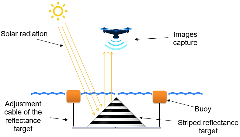
Figure 1 Illustration of a capture device that uses a graduated cone to quantify the water transparency of fishponds.
Cables are anchored into four buoys and attached to the cone, so that its tip can be aligned with the water surface to allow accurate measurements. Furthermore, those accessories allow the cone to be easily moved, as necessary.
To capture the images, a prototype was built with an ARMv8 64-bit processor operating at 1.2GHz, 1GB of LPDR2 SDRAM, input and output card drives, and two serial interfaces specially designed to capture images simultaneously, which were attached to 2 Sony sensors model IMX219 with a resolution of 3280 x 2464 (8 megapixels). An operating system based on Debian Linux was installed on the device, and a program was developed to manage the sensors, capture the images, and store them along with their metadata, such as date and time, geographic position, RPAS direction, and environment lighting at the time of the capture. All electronic components were assembled in a case designed with Thinkercad (a free 3D modeling software) and printed on a 3D printer using 1.75mm PLA filament at a temperature of 210 degrees Celsius.
The first sensor was prepared to capture near infrared (NIR) images (wavelengths ranging between 700 and 2500 nanometers) by attenuating wavelengths below 720 nanometers, thus eliminating the visible light range (whose wavelengths range from 400 to 700 nanometers). The second sensor was prepared to capture visible light, so it was endowed with a band pass filter that rejects anything that is not in the red (R), green (G) and blue (B) spectra (respectively, the bands between 600 and 700 nanometers, 500 and 600 nanometers, and 400 and 500 nanometers).
By configuring the sensors this way, the spectral response of the images captured can be analyzed in four different bands (NIR, R, G and B), thus allowing one to choose the most appropriate band to estimate the turbidity of a body of water according to the circumstances.
2.2. Procedures to evaluate the prototype operation
After the equipment was properly assembled and configured, the water bodies of 11 excavated ponds located in a rural area of Toledo city, PR - Brazil (coordinates -24.696540°, -53.779778°), were analyzed through 66 aerial images. A Google Earth view of this area is shown in Figure 2.
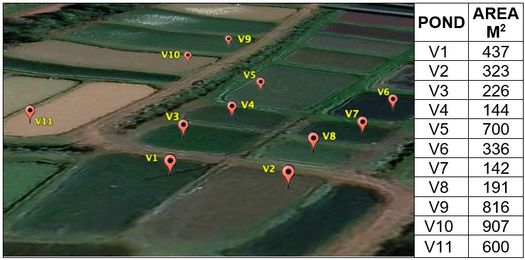
Figure 2 Excavated ponds of fishing farm of a rural producer in the city of Toledo - PR where samples were collected for water transparency analysis. Map source: Google (2020).
The data gathering took place on December 26th, 2020, between 10 am and 02 pm, when the sky was clear, with few clouds and little wind. The transparency of the water of all ponds was measured by using a 30-centimeter Secchi disc right before the prototype started to take pictures of the same areas.
The prototype was attached to an RPAS model “Phantom 4 Advanced” manufactured by DJI, which flew over the ponds at an altitude of 5 meters. In this experiment, a single cone was used in all ponds, so it had to be washed right before it was moved from one pond to another (to avoid any reflection disturbances). Six shots were taken from each pond and later transferred to a desktop computer for further processing and analysis
2.3. Image Processing
To analyze the images taken by the prototype, a program was developed in Python and Open Computer Vision library (OpenCV, 2015). First, the image is converted into a grayscale, a format in which each pixel is a single sample representing a given light intensity ranging from 0 to 255. Afterwards, the noise in the resulting picture is filtered with a convolution matrix that normalizes each pixel according to its neighboring pixels. Finally, the geometric shape of the target (the cone) is detected in the images by using the Hough transform (Hough, 1962).
Once the cone is detected, the image is segmented from its tip in order to create a new image 800 pixels high and 800 pixels wide, thus reducing the search space for the next processing stages. The dimensions of those segments are equivalent to the cone framing in images captured at altitudes of 3 meters or more.
The next processing stage performs pixels binarization - each pixel becomes white or black according to an adaptive threshold, which is the average of a set of pixels relative to its neighboring pixels. This process is important to tell the white stripes of the cone from the black ones, so that they can be counted despite the interference of the water surface.
In the last stage, the tonal variations of the pixels are analyzed, starting from the tip of the cone, in 4 orthogonal directions. This procedure is twofold: it detects where the visible stripes of the cone end and filters out interferences that were not eliminated in the prior stage, e.g., high intensity reflections that do not have a striped pattern. Given that the prototype took images from different angles, some stripes may be more visible in one direction than another, so it was defined that the final count would be the statistical mode among the counts in the 4 directions (top, bottom, left and right).
Finally, the number of stripes recognized in the image was multiplied by 4, which is the width of each one of them, resulting in a value in centimeters corresponding to the Secchi depth.
2.4. Efficiency analysis
After the algorithm was developed, it was used to process the 66 images captured in the field in 5 different spectral arrangements: near infrared (NIR), red (R), green (G), blue (B) and RGB, the later resulting from the combination of the R, G and B bands. These estimations were recorded on a spreadsheet and then statistically compared with the data gathered via the Secchi disk, so that the accuracy of the measurements provided by each spectral band could be computed.
The Shapiro-Wilk test confirmed that the data were normally distributed, which allowed us to employ the Pearson's linear parametric analysis to verify if there was a significant statistical difference among the estimates coming from both sensors, considering α = 0.05. All the statistical tests were conducted using the R environment (R CORE TEAM, 2018) and the complementary statistical package “agricolae” (de Mendiburu, 2017).
3. Results and discussion
3.1. Description of the equipment
The case of the prototype was designed to be carried through the air by an RPAS “Phantom 4 Advanced” manufactured by DJI, as shown in Figure 3.

Besides the HDMI, USB and ETHERNET interfaces that enable communication with a desktop computer (needed for data and programs transferring), the prototype is also endowed with a micro-USB port that allows it to be recharged using an ordinary phone charger (when its battery is full, the RPAS has an autonomy of 3 hours approximately). Two communication interfaces are connected to a compass and a digital luxmeter located above the propellers to mitigate interferences. A serial port can send messages informing the status of the shots (successful/unsuccessful) besides enabling the operator to capture images remotely. Alternatively, the prototype can be programmed to take pictures periodically according to an adjustable period.
The cone was placed withing the ponds, hung with 3 mm nylon ropes to four buoys made of tubular pet bottles. By adjusting the length of the ropes, the cone can be positioned correctly, with its tip leveled with the surface of the water as seen in Figure 4.

3.2. Images processing
We developed a single algorithm to process the images captured in the NIR, R, G and B bands. It was designed for maximum performance under real usage scenarios, i.e., considering adverse conditions such as reflexes, waves, and bank vegetation.
Figure 5 shows an image that was gathered on field and converted to a grayscale (a), normalized with an adaptive thresholding process (b), and then had the tip of the cone identified with the Hough transform (c). Note that false positives were not identified in this example.
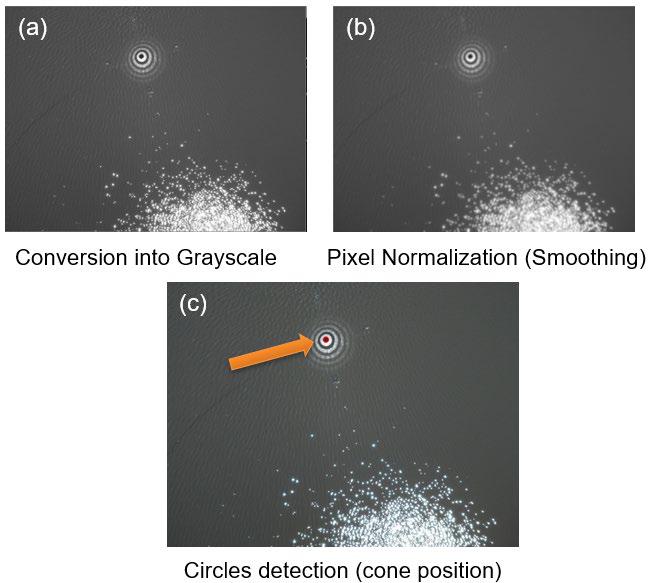
Figure 5 Reference cone for aerial images, for the purpose of analysis of the bodies of water transparency in a fishpond.
Given the conditions in which the shots were taken, the cone detection procedure was outstanding: its tip was painted by a black circle of only 95 mm in diameter and the images were captured at an altitude of 5 meters. In other works, much larger targets (diameters bigger than 25 cm) are needed for pictures taken at this same altitude (Alsalam et al., 2017).
Once the coordinates of the cone have been determined, its surrounding areas may be discarded, and then the image can be binarized so the stripes can be identified and counted as shown in Figure 6.
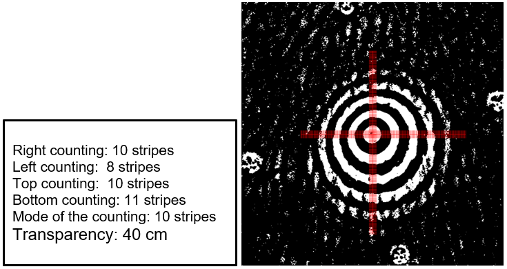
Figure 6 Extraction, binarization, and counting of the cone's stripes in four directions (right, left, top and bottom).
There is a significant noise in Figure 6, perceived as reflections and waves with diameters and colors that are like the white stripes of the cone, which could occasionally lead to false positives. Given that the noisy areas are badly fragmented, and the actual stripes are near-contiguous in the pictures, false positives are mitigated by a simple normalization procedure we created and named as “capillary scanning”: several imaginary lines irradiating from the tip of the cone are traced in the image and segmented in groups of four pixels, which are traversed by orthogonal lines 10 pixels long. In case the orthogonal strings are similar in intensity to the segments, then the continuity of that area is declared.
The scanning was necessary because aquatic surfaces are prone to the formation of waves that reflect the sunlight, forming shapes that blend with each other (a pattern known as “salt and pepper”). This is a common issue that plagues the research of image processing in aquatic environments - many practitioners are aware that it is a thankless task to remove those noisy patterns via the standard solution (moving average filters) as reported, e.g., in (Azzeh, 2018; Erkan et al., 2018). In turn, this issue was properly dealt with via the capillary scanning we propose in this work.
The altitude of the RPAS is also a critical tuning parameter that may require some attention and experience to be properly adjusted. For example, Peña et al. (2013) recommend that the shots be taken at an altitude of 30 meters to grant a broader view of the area under analysis, but in their case the goal was to identify weeds amidst a corn plantation. In fish farming however, there is no need for such a broad view of the ponds: an altitude of 5 meters is sufficient to analyze the transparency of their water bodies and prevents the propellers of the RPAS from causing additional waves on the surface of the ponds, besides protecting the equipment from the moisture.
The angle of the images capture can also impact the stripes detection and counting, as highlighted in Figure 6. In the left counting, the drone inclination made the algorithm to identify 2 stripes less than in the right and top countings. However, thanks to the 4-directions scanning, the algorithm was able to determine the correct amount of visible stripes (ten) by using the statistical mode of all countings. This robust though simple procedure makes it unnecessary to take impeccable shots with the RPAS steady in an optimal inclination - an idealized condition that is hardly found in the field.
3.2. Efficiency analysis
After all images were processed, the results were recorded in a spreadsheet as seen in Table 1.
Table 1 Results of the transparency analyses obtained with a Secchi disc and the corresponding estimates obtained by the proposed algorithm.
| POND | SECCHI DISC (cm) | NIR BAND RESULT (cm) |
RGB
BAND RESULT (cm) |
R
BAND RESULT (cm) |
G
BAND RESULT (cm) |
B
BAND RESULT (cm) |
| V1 | 31 - 31 - 31
31 - 31 - 31 |
32 - 32 - 32
32 - 32 - 32 |
24 - 24 - 24
28 - 28 - 28 |
24 - 24 - 24
24 - 28 - 24 |
24 - 24 - 28
28 - 28 - 28 |
04 - 08 - 16
28 - 16 - 16 |
| V2 | 25 - 25 - 25
25 - 25 - 25 |
24 - 24 - 24
24 - 24 - 24 |
08 - 16 - 16
16 - 16 - 16 |
24 - 24 - 24
24 - 24 - 24 |
08 - 16 - 16
16 - 16 - 16 |
60 - 08 - 56
44 - 44 - 08 |
| V3 | 38 - 38 - 38
38 - 38 - 38 |
40 - 40 - 40
40 - 40 - 40 |
24 - 28 - 40
36 - 24 - 24 |
36 - 24 - 24
36 - 32 - 28 |
24 - 24 - 28
24 - 24 - 24 |
24 - 24 - 24
28 - 24 - 32 |
| V4 | 39 - 39 - 39
39 - 39 - 39 |
40 - 40 - 40
40 - 40 - 40 |
28 - 32 - 32
32 - 32 - 32 |
32 - 32 - 32
32 - 32 - 32 |
24 - 28 - 28
28 - 28 - 32 |
28 - 24 - 24
24 - 24 - 24 |
| V5 | 38 - 38 - 38
38 - 38 - 38 |
40 - 40 - 40
40 - 40 - 40 |
24 - 24 - 24
24 - 24 - 24 |
32 - 32 - 32
32 - 32 - 32 |
24 - 24 - 24
24 - 24 - 24 |
16 - 12 - 12
12 - 12 - 12 |
| V6 | 30 - 30 - 30
30 - 30 - 30 |
32 - 32 - 32
32 - 32 - 32 |
24 - 24 - 24
24 - 24 - 24 |
24 - 24 - 24
24 - 24 - 24 |
24 - 24 - 24
24 - 24 - 24 |
08 - 08 - 64
64 - 08 - 08 |
| V7 | 41 - 41 - 41
41 - 41 - 41 |
40 - 40 - 40
40 - 40 - 40 |
32 - 32 - 32
32 - 32 - 32 |
32 - 32 - 32 32 - 32 - 32 |
32 - 32 - 32 32 - 32 - 32 |
48 - 24 - 24 24 - 24 - 24 |
| V8 | 43 - 43 - 43 43 - 43 - 43 |
40 - 40 - 40 40 - 40 - 40 |
32 - 32 - 32 32 - 32 - 32 |
32 - 36 - 32 32 - 36 - 32 |
32 - 32 - 32 32 - 32 - 32 |
24 - 24 - 24 24 - 24 - 24 |
| V9 | 33 - 33 - 33 33 - 33 - 33 |
32 - 32 - 32 32 - 32 - 32 |
24 - 24 - 24 24 - 32 - 28 |
28 - 24 - 28 32 - 24 - 24 |
24 - 24 - 24 24 - 36 - 32 |
16 - 28 - 28 24 - 36 - 28 |
| V10 | 33 - 33 - 33 33 - 33 - 33 |
32 - 32 - 32 32 - 32 - 32 |
32 - 32 - 32 32 - 32 - 32 |
40 - 36 - 36 36 - 36 - 36 |
32 - 32 - 32 32 - 32 - 32 |
24 - 28 - 24 24 - 24 - 24 |
| V11 | 07 - 07 - 07 07 - 07 - 07 |
08 - 08 - 08 08 - 08 - 08 |
08 - 28 - 08 08 - 08 - 08 |
08 - 24 - 08 08 - 08 - 08 |
08 - 24 - 08 24 - 08 - 08 |
44 - 32 - 08 48 - 08 - 44 |
The measurements obtained with the Secchi disk were compared with those estimated by the algorithm through the images. The Shapiro-Wilk test shown in Figure 7 indicates that these data followed a normal distribution with no outliers.
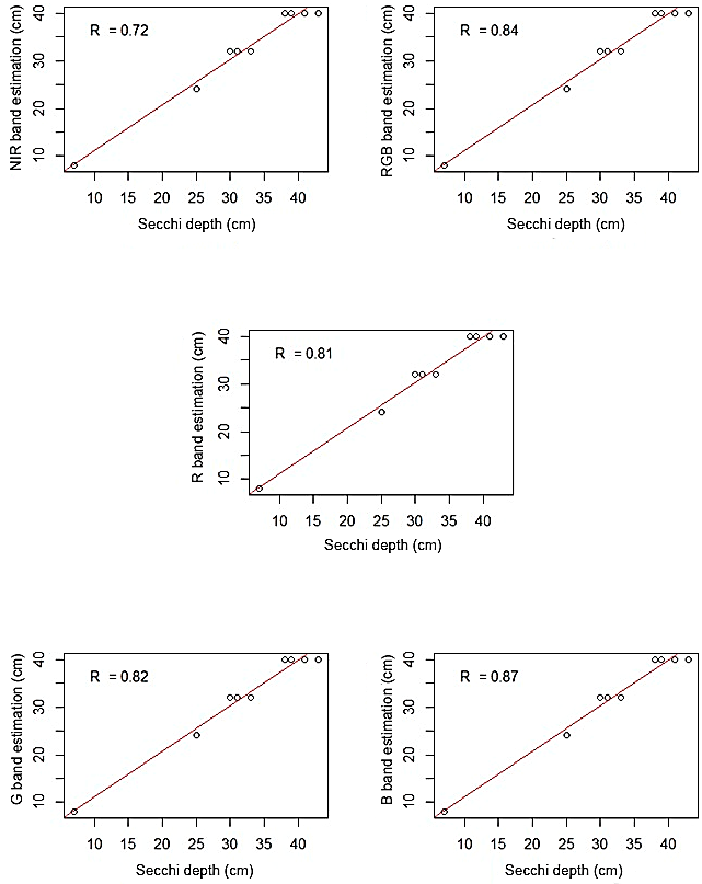
Figure 7 Distribution of the data estimated for the NIR, RGB, R, G and B bands regarding the measurements made with a Secchi disc.
A Pearson's correlation test unveiled a strong positive correlation (r = 0.9861427, n = 11 with 6 repetitions per variable) between the measurements made with the Secchi disk and the estimates made with the NIR band of the images. Significant correlations were also got by using bands R (r = 0.8409687), RGB (r = 0.7917608), G (r = 0.7355359).
Other studies that propose estimation of the water transparency by multispectral images without the use of reflective targets report lower correlations than those we got in this work. For example, Prior et al. (2020) obtained a maximum correlation of 0.78, and Mceliece et al. (2020) obtained a correlation of 0.74. Those results suggest that the analysis of reflectance based on fixed targets is less sensitive to interference when compared to direct reflectance. Briefly, the usage of the reflective cone was essential to grant the superior results we are reporting here.
As a rule, highly transparent waters reflect little visible light and no infrared light. However, Cahyono et al. (2019) observed that as the occurrence of suspended particles increases, the water transparency decreases. Herewith, there is also a change in the reflectance levels of the R band between 600 and 700nm, and of the NIR band between 750 and 1400nm (Song et al., 2012; Amanollahi et al., 2017). This phenomenon was also observed in this work.
Still according to Cahyono et al. (2019), high concentrations of chlorophyll arising from algae reflect mainly the G band, between 500 and 600nm, suggesting that higher wavelength bands (above 600nm) are not so affected by the reflectivity of the water and plants, but they might be blocked by solid particles that make the water look turbid. This is corroborated by Lotfi et al. (2019), Pereira et al. 2021), who also observed a greater correlation between water transparency and the levels of reflectance in the band R when compared to the B band.
This was also observed in this work: the images processed in the NIR, and R bands had a higher hit rate than the ones processed in other bands. Moreover, the R band presented a lower transparency than the estimate made in the NIR band in 64% of the images analyzed. This shows that the smaller the wavelength, the greater are the interferences that prevent the noise (waves around the cone) from reaching the optical sensor, which makes sense given that the light needs to traverse the water, reflect on the cone and reach the optical sensor - a long path in which the light can be blocked or even irradiated to different directions.
Given that the cone was 40 cm high, that was the maximum depth the developed algorithm managed to estimate. This limitation affected the estimations gathered in the pond number 8: the transparency measured by the Secchi disk was 43 centimeters and the estimate was only 40 centimeters. However, a higher cone featuring more stripes could easily solve that issue. In the other ponds, the water transparency fell within the range of 40 centimeters depth and the estimates were accurate as expected, with an error margin of 2 centimeters in the NIR band.
The stripes of the cone used in this experiment were 4 centimeters wide, which means that the estimates are subject to errors that are multiples of 4 because they are based on stripe counts. However, these “natural” error margins are excellent when compared to methods based on water reflectance, as proposed by Pereira-Sandoval et al. (2019). In that case, the accuracy was 88 centimeters on a Secchi transparency scale ranging from 0.26 to 8.1 meters and the images were captured by the Landsat OLI satellite. According to Castro et al. (2020), the use of images captured by RPAS improves the space-temporal resolution when combined with satellite images. Anyway, the fact is that satellite-based analyses are not ideal for fishponds, due to their lower resolution and inferior colors definition. The use of shots taken with an RPAS provides superior results.
4. Conclusions
The prototype and algorithms we developed proved to be accurate and robust to estimate the transparency of water bodies of fishponds. They are also inexpensive, given that the prototype was equipped with optical sensors that cost less than US$ 150 dollars. The images gathered in the field had a quality sufficient for our image processing algorithms and no interference caused by the RPAS (e.g., vibrations) were observed, which is remarkable given that the image capture sensors had no dampening systems. The prototype has computing capabilities that enable it for real-time image processing, so transparency estimates can be transmitted to other systems during flights if needed. Estimates are more accurate with wavelengths above 720nm, a band in which they feature a maximum error of 5%. However, shorter wavelengths provide less accurate estimates.

