


 nueva página del texto (beta)
 Inglés (pdf)
 Artículo en XML
 Referencias del artículo
 Enviar artículo por email
 Citado por SciELO
  Similares en
SciELO
Similares en
SciELO 
 Permalink
Introduction
A permeable reactive barrier (PRB) is an effective remediation technology for contaminated groundwater with diverse compounds, including chlorinated ethenes, that require careful design prior to field installation (Blowes et al., 2000; Bone, 2012; Careghini, Saponaro, & Sezenna, 2013; Gavaskar, Gupta, Sass, Janosy, & Hicks, 2000; Powell et al., 1998; Thiruvenkatachari, Vigneswaran, & Naidu, 2008). Two main PRBs configuration types for field applications are commonly used: the funnel-and-gate and the continuous wall systems (Powell et al., 1998; Thiruvenkatachari et al., 2008). The continuous wall system allows the flow of the contaminant plume through the whole width of the reactive wall. The funnel and gate system consists of impermeable walls, which direct the contaminant plume to the permeable gate(s) filled with selected contaminant-specific reactive materials.
Groundwater models have been used in most PRB installations to determine the approximate location of the reactive wall with respect to the contaminant plume movement (Courcelles, 2015; Garon, Schultz, & Landis, 1998; Gupta & Fox, 1999; Kimmel et al., 2003; Painter, 2004; Scott & Folkes, 2000). Models are usually set up after laboratory tests have estimated the contaminant degradation rates and the residence time requirements depending on the selected reactive materials (Gavaskar et al., 2000; Gupta & Fox, 1999). Numerical groundwater flow and transport modeling is an important tool for incorporating the site-specific hydrogeology into the design and optimization of PRBs (Gupta & Fox, 1999). Such models allow for understanding groundwater flow paths and volumes so one can simulate different input parameters to determine the suitable location, configuration of the PRB, and the thickness of the reactive gate. The modeling process prevents over-cost of gates that are too long or thick or not placed in optimal locations. In addition, the selection of monitoring points can be possible with an understanding of the resulting flow system after the installation of the PRB. Evaluation of possible difficulties such as seasonal fluctuations of groundwater flow direction and changes in hydraulic properties of the reactive material over time can also be predicted with modeling (Gavaskar et al., 2000; Scott & Folkes, 2000).
Important parameters such as hydraulic capture zone and residence time need to be addressed during the modeling process. The hydraulic capture zone refers to the width of the zone of groundwater that will pass through the gate rather than under, over or around the barrier (Bekele, Naidu, Birke, & Chadalavada, 2015; Gavaskar et al., 2000; Muguet, Cosme, & Vermeiren, 2004). The residence time refers to the time the contaminant will be in contact with the reactive material in the reactive gate (Gavaskar et al., 2000).
Groundwater models can be classified based on spatial dimension from 1-D to 3-D. They can be either steady state or transient (time dependent). In addition, models can be limited to groundwater flow or consider solute transport as well. Several computer codes are available to evaluate groundwater flow through PRBs, including (among others): MODFLOW (McDonald & Harbaugh, 1988), FLONET/TRANS (Guiguer, Molson, Frind, & Franz, 1991), GMS (EMRL, 2000), FEFLOW (Diersch, 2002). MODFLOW is a well-known and commonly used code in PRBs applications (Courcelles, 2015; Elder, 2002; Harte, Konikow, & Hornberger, 2006; Kimmel et al., 2003; Lin, Benson, & Lawson, 2005; Painter, 2004). It uses a finite difference method to represent the hydrogeological properties in the model domain (Guiguer & Franz, 1996).
This paper presents the design and evaluation of a PRB to treat TCE contaminated groundwater with the aid of the modeling code MODFLOW (Guiguer & Franz, 1996). The developed model was used to test various PRB configurations and select the most effective system to treat groundwater contaminated with trichloroethene (TCE) in the vicinity of Nowa Dęba (South-East Poland). The simulations were based on the hydraulic capture zone, residence time and the water volumes through the reactive wall. Although, this kind of work has been done before in different PRB applications (e.g., Garon et al., 1998; Gupta & Fox, 1999; Kimmel et al., 2003; Scott & Folkes, 2000), there are only few published papers addressing the modeling part of the design process.
Methods
Site conditions and hydrogeology
The contaminated site is located in Southeast Poland and covers an area of approximately 30 km2. Site-specific hydrogeology and stratigraphy were evaluated from a total of 39 wells and piezometers. The aquifer is mainly composed of quaternary alluvial and terrace deposits of sand, silt, clay and gravel with depths up to 30 m below the ground surface (bgs). The unconfined aquifer lies on an impervious layer of Miocene clay deposits and Carboniferous rocks that extends hundreds of meters bgs. The water table is located from 0.5 to 16.5 m bgs. The groundwater table fluctuates seasonally with variations no greater than 0.8 m. The groundwater flows in a northwest direction at a seepage velocity of 0.4 m/d with a horizontal gradient of about 0.05. The groundwater flow regime is influenced by the water extraction wells of a nearby waterworks. The hydraulic conductivity falls in the range of 1 x 10⁻⁷ to 4 x 10⁻⁴ m/s as assessed from an aquifer-pumping test conducted on 31 wells located at the site (Szklarcyk, Kret, Grajales-Mesa, Kiecak, & Malina, 2012).
Historic releases of chlorinated solvents from a former metalwork and ammunition factory came into contact with and dissolved into groundwater, resulting in a groundwater plume that has migrated in a northwest direction into the extraction wells of a waterworks. Groundwater chemical analysis indicates the concentrations of TCE up to 6 130 μg/L, exceeding the maximum concentration limits (MCL) established in the Polish regulation (5 μg/L) (Kret, Kiecak, Malina, & Szklarcyk, 2011). The location of the plume in relation to the site is shown on Figure 1. Containment and treatment of the groundwater plume by installing a PRB in the northwest portion of the site was suggested (Kiecak, Malina, Kret, & Szklarczyk, 2017).

The model development and set up
The development of the model included the following sequential steps: 1) hydrological characterization of the site; 2) construction of the conceptual model; 3) selection of the computer code; 4) translation of the conceptual model into the mathematical model (input parameters); 5) calibration; 6) predictive simulations.
The hydrological characterization of the studied site included a complete field campaign and laboratory studies (batch and column experiments). Afterwards, desk studies were performed for the interpretation of the collected data.
With the data collected a conceptual model was constructed. The conceptual model was a three-dimensional representation of groundwater flow and contaminant transport, and thus included all available geologic, hydrogeologic, and geochemical data from the site.
After hydrogeological characterization of the site was completed and the conceptual model developed, computer software was selected. The computer code should be capable of simulating conditions at the studied site. Analytical models for example are used where the field data shows that the groundwater flow or transport processes are relatively simple. Numerical models one, two or three-dimensional are selected based upon the hydrogeological characterization and model conceptualization. For the present work, a three-dimensional (3-D), finite-difference visual MODFLOW model (Guiguer & Franz, 1996) was developed to simulate the performance of a PRB in the studied aquifer.
The governing equation for three-dimensional flow in saturated porous media for MODFLOW is described by the partial differential equation:
Where K xx , K yy , and K zz are the values of hydraulic conductivity along the x, y and z coordinates; h is the potentiometric head; W is the volumetric flux per unit volume representing sources and sinks; S s is the specific storage of the porous medium, t is time.
The MODFLOW software represents the aquifer system with cells using a sequence of layers and a series of rows and columns. The software solves the finite-difference equations simultaneously using one of several numerical solver algorithms and accounts for groundwater flow between cells and between cells and external sources or sinks of water, such as stream-aquifer hydraulic interaction, aquifer recharge, or groundwater withdrawal by wells. Aquifer properties are assumed to be uniform within each model cell, and hydraulic heads are assumed to be at the center of each cell.
With the computer code selected, the input parameters like model grid size and spacing, layer elevations, boundary conditions, hydraulic conductivity, recharge, definition of the sources and sinks (lakes, rivers, extraction wells) were selected.
The modeled area consisted of 23.75 km2 of active cells discretized in a grid of 30 m by 30 m size and five layers of different thickness to represent the heterogeneous aquifer (Table 1). Each of the five layers was simulated with the same number of active blocks.
Table 1 Model parameters (derived from Szklarcyk et al., 2012).
| Layer number | Geological Unit | Aquifer type | Thickness (m) | Porosity (-) | Hydraulic conductivity (m/s) |
|---|---|---|---|---|---|
| 1 | Fine to medium grained sands | Unconfined | 25 | 0.28 | 2.064 x 10⁻⁵ |
| 2 | Gravel and varied-grained sands | Unconfined/confined | 19 | 0.31 | 2.98 x 10⁻⁴ |
| 3 | Fine-grained sands | Confined | 14 | 0.35 | 1.064 x 10⁻⁵ |
| 4 | Clay and silt | Confined | 13.6 | 0.40 | 1.0 x 10⁻⁷ |
| 5 | Gravels | Confined | 19 | 0.25 | 4.0 x 10⁻⁴ |
Hydraulic conductivity changes on the investigated area were described based on data compiled by the Polish Geological Institute in the Bank HYDRO database (PGI-NRI, 2010). Hydraulic conductivities from this database were collected from pumping test performed to a 31 wells and piezometers located on the site. For the present work a specific value of hydraulic conductivity was assigned to each of the five layers of the model. For the case of layer four, the hydraulic conductivity value was taken from literature - as a typical value for non-permeable soils: clays and silts. Variability of hydraulic conductivity for all model layers in the aquifer is shown in Table 1.
In the construction of the model boundary conditions of first kind (Dirichlet), second kind (Neumman) and the third time (Cauchy) were adopted. Constant head boundary conditions (Dirichlet) were assigned at the north and south boundary to simulate the lateral inflow and outflow of groundwater to and from the model. Constant flux boundary conditions (Neumman) were assigned to simulate water extraction from the wells at the waterworks and also to simulate recharge from infiltration. Mixed boundary conditions (Cauchy) were assigned to simulate the influence of surface water bodies (Dęba, Bystrzyk, Koniecpolka) on the groundwater flow.
Groundwater recharge by infiltration of precipitation in the Nowa Dęba area is of 847 mm from which 20-25% is infiltrated into the soil. Based on this estimate, a uniform recharge rate of 200 mm per year was used in the groundwater flow model. Groundwater withdrawal at the site ranged from 73 to 1 240 m3 /d since the aquifer is the main source of drinking water for municipal, commercial and industrial uses in the town of Nowa Dęba.
Calibration of the model was done with data collected in 2010 from 39 observation points. The correlation coefficient of the model was 1 and the highest difference of observed and calculated hydraulic head was of 0.5 m. For a complete description of the numerical groundwater flow model refer to Szklarcyk et al. (2012).
Once the groundwater flow model was calibrated, the contaminant transport model was simulated using the MT3DMS code for MODFLOW. The initial TCE concentrations in the model were estimated from observation and production wells at the site. Laboratory tests were used to determine transport parameters like sorption and biodegradation rate (Kret, Kiecak, Malina, Nijenhuis, & Postawa, 2015).
Finally, the PRB systems were modeled for the continuous barrier and for the funnel and gate system. From the plume delineation it was recognized that a PRB of a minimum 1 000 m in length was needed. The simulated PRBs were fully penetrating, keyed to an impermeable layer and located perpendicular to the groundwater flow. In the area where the PRB was simulated the grid was discretized to 1 m by 1 m. The funnel (slurry wall) was simulated using the Horizontal Flow Barrier Module feature of MODFLOW, having a K of 9 x 10⁻⁹ m/s. The reactive gate consisting of a mixture of compost - brown coal (1:3 by weight) was first simulated with two K values: one determined during laboratory experiments and one measured during the field experiments (5 x 10⁻⁴ and 3 x 10⁻⁵ m/s, respectively) (Grajales-Mesa & Malina, 2016; Grajales-Mesa & Malina, 2019). All funnels were set at 180°. According to the works of Starr and Cherry (1994) , the flow in the gate is maximum for an angle of walls of 180°.
The capture zone width in each of the simulations was determined by tracking particles forward through the reactive gate with the MODPATH code (Pollock, 1989). Particles were added upstream of the barrier along a 3 000-m-long line. The location of the flow divides between particles passing through the reactive gate and those passing around the ends of the funnel were used to determine capture zone width. Residence time within the reactive gate for each simulation was determined from the time required for the particles to pass through it. From our laboratory and field experiments it was concluded that a residence time of at least three days is required for the site to reduce TCE concentration to acceptable values. In addition, the discharge through the reactive gate was calculated with the ZONE BUDGET package (Harbaugh, 1990).
Because chlorinated solvents are expected to persist for long periods of time and it is known that reactions within the barrier result in formation of inorganic precipitates, it is necessary to estimate for how long the PRB will retain its permeability. Thus, additional simulations were conducted to evaluate the effects of decreased permeability of the gate over its period of operation; following the work of (Gupta & Fox, 1999) the hydraulic conductivity of the reactive material, K PRB was reduced in 10% increments from the initial 5 x 10⁻⁴ to 5 x 10⁻⁶ m/s. For each individual simulation, the same values for K aq (hydraulic conductivity of the aquifer) were used.
A total of 60 simulations for different PRB design scenarios incorporating variable funnel and gate lengths, variations in number and position of gates (simulations 1-24; Table 2) as well as changes in K PRB (simulations 25-60) were run.
Table 2 Summary of the different PRBs configurations simulated in this study.
| Scenario | number of funnels | number of reactive gates | funnel width (m) | gate width (m) | gate thickness (m) | K PRB (m/s) |
|---|---|---|---|---|---|---|
| 1 | 0 | 1 | 0 | 1 000 | 1 | 0.0005a |
| 2 | 2 | 1 | 360 450 | 500 | ||
| 3 | 3 | 2 | 180 | 330 | ||
| 4 | 4 | 3 | 120 | 240 | ||
| 5 | 0 | 1 | 0 | 1 000 | 2 | |
| 6 | 2 | 1 | 360 450 | 500 | ||
| 7 | 3 | 2 | 180 | 330 | ||
| 8 | 4 | 3 | 120 | 240 | ||
| 9 | 0 | 1 | 0 | 1 000 | 3 | |
| 10 | 2 | 1 | 360, 450 | 500 | ||
| 11 | 3 | 2 | 180 | 330 | ||
| 12 | 4 | 3 | 120 | 240 | ||
| 13 | 0 | 1 | 0 | 1 000 | 1 | 0.00003b |
| 14 | 2 | 1 | 360, 450 | 500 | ||
| 15 | 3 | 2 | 180 | 330 | ||
| 16 | 4 | 3 | 120 | 240 | ||
| 17 | 0 | 1 | 0 | 1 000 | 2 | |
| 18 | 2 | 1 | 360, 450 | 500 | ||
| 19 | 3 | 2 | 180 | 330 | ||
| 20 | 4 | 3 | 120 | 240 | ||
| 21 | 0 | 1 | 0 | 1 000 | 3 | |
| 22 | 2 | 1 | 360, 450 | 500 | ||
| 23 | 3 | 2 | 180 | 330 | ||
| 24 | 4 | 3 | 120 | 240 |
aK value measured during laboratory experiments (Grajales-Mesa & Malina, 2016).
bK value measured during field experiments (Grajales-Mesa & Malina, 2019).
Results and discussion
Evaluation of simulated PRBs scenarios
The selection of the best PRB configuration requires a careful examination of different alternatives’ pros and cons and their cost implications. In general terms, the ideal design should be able to capture the entire plume, minimize the thickness of the barrier and the number of gates while being able to provide adequate residence time (Suthersan, Horst, Schnobrich, Welty, & McDonough, 2016).
The evaluation of the model results (Table 3) to select the most effective PRB design was performed considering the following criteria:
The entire plume passes through the reactive gate.
Absence of end flows around the reactive gates and funnel walls.
No flows under or over the reactive gates and funnel walls.
Minimum thickness for the desired residence time (three days).
Minimum number of gates.
Costs.
Table 3 Results for the simulated scenarios.
| Scenario | Flux through the gate (m3/s) | Capture zone (m) | Residence time (days) |
|---|---|---|---|
| 0 | - | - | - |
| 1 | 2 687.68 | 925.532 | 1 |
| 2 | 2 506.047 | 903.448 | 1 |
| 3 | 2 705.34 | 995.455 | 1.2 |
| 4 | 2 833.656 | 1 028.571 | 1.2 |
| 5 | 2 666.989 | 932.432 | 2.1 |
| 6 | 2 483.641 | 876.923 | 2 |
| 7 | 2 658.651 | 990.91 | 1.5 |
| 8 | 2 809.044 | 1 017.857 | 1.7 |
| 9 | 2 651.517 | 923.684 | 3.7 |
| 10 | 2 468.824 | 879.07 | 3 |
| 11 | 2 655.263 | 980 | 2.5 |
| 12 | 2 790.183 | 1 041.667 | 3 |
| 13 | 2 269.045 | 911.688 | 1.5 |
| 14 | 2 137.765 | 888.312 | 1 |
| 15 | 2 273.938 | 945.652 | 1 |
| 16 | 2 390.017 | 990 | 1 |
| 17 | 2 055.703 | 788 | 3.2 |
| 18 | 1 905.366 | 771.428 | 2.3 |
| 19 | 2 023.78 | 810.811 | 2.3 |
| 20 | 2 131.255 | 867.568 | 2.4 |
| 21 | 1 914.511 | 780.822 | 5.6 |
| 22 | 1 763.798 | 694.737 | 4 |
| 23 | 1 859.537 | 786.486 | 4.1 |
| 24 | 1 969.518 | 757.895 | 4 |
Figure 2 presents the selected simulation results of the capture zones for studied barrier configurations.

Effects of barrier’s dimension and configuration on the capture zone width
Form the results it can be noted that capture zone width ranged from 1 041 to 694 m. Comparison of the particle flow paths for different scenarios (Figure 2 and Figure 4) demonstrates the usefulness of modeling in the PRB design process. When comparing the scenario without PRB (Figure 2a) to the scenario with a continuous barrier (Figure 2b), there is not much difference in the flow paths although the contaminant plume passes through the reactive gate in the continuous barrier. This suggests that the water is directed towards the gate mainly due to the effect of the extracting wells located downgradient of the barrier. Figures 2c to 2e clearly show how the funnels contribute to direct contaminated groundwater towards the reactive gate. In addition, when more funnels are added there is an increase in the flow through the gate and the capture zone width. As pointed by other authors, in funnel and gate systems capture zone extends from half of the funnel wall width at each side (Gupta & Fox, 1999). Although the capture zone for a PRB at a heterogeneous site was expected to be highly asymmetrical and with significant differences in residence time at different depths (Gupta & Fox, 1999), it was not in our case, possibly due to the influence of the extracting wells downgradient of the barrier as pointed out earlier in this section. It is evident that the aquifer heterogeneities had little impact on the symmetry of the capture zone. In addition, the location of the barrier in a zone of high hydraulic conductivity was an advantage, since it forms preferential pathways for most of the flow and directs the contaminant plume towards the reactive gate (Gavaskar et al., 1997). The particles released in the area showed movement through the reactive gate that varied from 1 to 5 days with small increases in residence time to the ends of the gate where the hydraulic conductivity of the aquifer is lower.
In addition, the simulated changes in barrier thickness did not result in significant differences in the capture zone width and discharge through the gate. It implies that for this site the capture zone width changes according to the number and location of the funnel walls but is not affected by the thickness of reactive gate. In contrast, Garon et al. (1998) concluded that capture zone decreases with increasing PRB thickness due to greater resistance to flow. And for a given PRB thickness, capture zone increases with increasing PRB width due to changes in flow gradient that is greater in the center of the barrier than the gradient tangent to the PRB. Differences in geogoly and hidrogeology at the studied sites may explain the discrepancy between the results presented here and Garon et al. (1998).
As expected, the residence time increased as the barrier thickness was increased. However, increasing the barrier thickness to achieve a longer residence time represents higher costs.
Effects of the hydraulic conductivity of reactive media on the capture zone width
All reactive barriers have a finite treatment capacity. Continuous flow of groundwater containing suspended fine particles clogs zones of the barrier even without any chemical reactions. In addition, chemical reactions and bacterial growth in PRBs cause fouling. Consequently, the hydraulic properties of PRBs changes during operation (Kacimov, Klammler, Il’yinskii, & Hatfield, 2011). In a PRB the hydraulic conductivity of the reactive material K PRB, is usually designed as K PRB > K aq . If K PRB is lower than K aq , groundwater will pass around the barrier, on the contrary if K PRB is higher than K aq groundwater will converge into the reactive gate. Moreover, the studies of Benner, Blowes, and Molson (2001) indicate that in a heterogeneous aquifer, the higher the K PRB the greater the preferential flow. Thus, designing a PRB in a heterogeneous aquifer where K PRB < K aq may be problematic because of the negative impact on capture zone.
Figure 3 shows that the capture zone width decreases as K PRB decreases at a given K aq . Reduction of K PRB from 5 x 10⁻⁴ to 5 x 10⁻⁶ resulted in a 54% decline in capture zone width and 65% reduction in discharge through the gate (Figure 3). When a decrease in K PRB is of one order of magnitude or greater it can be seen that the barrier is not able to capture the entire plume (Figure 4). This suggest that designing the barrier for this site with a reactive material of K PRB lower than that of the aquifer is not recommended as it will have a negative impact in the capture zone size and will not be able to capture the entire plume. This observation also evidences the importance of the replenishment of the material as porosity losses occur due to chemical reactions, adsorption into the material and bacterial growth causing change in the material properties during operation. In addition, a decrease in K PRB represents an increase in residence time (Table 3). Similar results were obtained on the simulations conducted by Liu, Li and Wang (2011). They showed that the capture zone width generally decreases with a decrease in K PRB at a given K aq . However, they observed that there is relatively little decrease in capture zone width when the K PRB of freshly installed reactive media is roughly 10 times higher than the K aq .
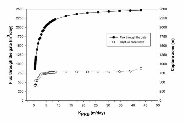
Figure 3 Discharge through the reactive gate and width of hydraulic capture zone as a function of reactive gate permeability.

Results indicate that the simulated reactive barrier was able to capture the contaminated plume when K PRB was at least 2 times higher than K aq (Figure 4). This means that for the studied site a reactive material with a K PRB of 0.00006 m/s or higher is required. In addition, the configuration with two funnels and one gate (3 m thick) is adequate for the site since it is able to capture the entire plume while minimizing the number of gates and providing the required residence time of three days (Scenario 10, Table 2). Nonetheless, an analysis of the estimated costs for the different configurations will give us additional criteria to take the final decision on the best barrier design.
Our results are consistent with results from Garon et al. (1998). They concluded that both the K PRB and the PRB thickness affect the capture zone.
Applications and limitations of the model
Numeric modeling of the groundwater flow field produced from the installation of a PRB should be considered as a prerequisite prior to developing the final design and installation of a PRB system. The results of model analysis can provide for a design that will optimize groundwater capture by incorporating multiple gates located along portions of the barrier, simulate different locations and predict the behaviour for the groundwater flow once the barrier has been installed. The thickness of the barrier can also be optimized to guarantee that the entire plume passes through the reactive gate, and to provide sufficient residence time of groundwater in the reactive barrier to accomplish treatment. Results from the particle-tracking model are essential in locating critical areas, where monitoring wells could be placed to assess performance of the system. The performance of the PRB over time can also be assessed by modeling the decrease in K PRB over time.
Despite its numerous advantages and applications, the model has some limitations. The most obvious one is that accuracy of the model predictions depend on the correctness of the model and uncertainty in model parameters. Because of the simplifying assumptions embedded in the mathematical equations and uncertainties in the values of data required by the model, a model must be viewed as an approximation and not an exact duplication of field conditions. In addition, models are site-specific, each groundwater flow model is unique and may require additional procedures in its development and application. For example, capture zone width results respond to a specific geometry and K PRB, and do not apply to all PRB applications. The model, however, even with site-specific restrictions, is useful for uderstanding the relationships between, geometry, K values and the capture zone width. Groundwater flow models, however, even as approximations are a useful investigation tool that groundwater hydrologists may use for a number of applications.
Cost considerations
The cost of PRB installation is a function of geology, hydrogeological conditions (i.e. aquifer thickness and depth), applied barrier configuration and construction methods. In general, the depth and the length of a PRB continue to drive the costs of a PRB application. The deeper the aquifer and the longer the PRB, the higher are the costs. Trenching may account for up to 70% of the total construction costs since it requires the mobilization of specialized equipment (AFCEE, 2008). Material costs are relatively inexpensive, on the order of 5-10% of the total installation costs; however, shipping to the site needs to be considered. Table 4 presents rough estimates for the costs of installation for different PRB systems simulated in our study.
Table 4 Summary of estimated costs of simulated PRB systems.
| Cost | Continuous | 1 gate | 2 gates | 3 gates |
|---|---|---|---|---|
| Reactive material (RM) | ||||
| Compost (20 US$/ton) | 490 000 | 245 000 | 323 400 | 352 800 |
| Brown coal (65 US$/ton) | 5 141 500 | 2 570 750 | 3 393 390 | 3 701 880 |
| Transport | 2 072 000 | 1 036 000 | 1 367 520 | 1 491 840 |
| Total RM cost (US$) | 7 703 500 | 3 851 750 | 5 084 310 | 5 546 520 |
| Construction and installation | ||||
| Funnel cost (US$) | 0 | 8 699 460 | 6 100 920 | 5 423 040 |
| Excavation and disposal cost (US$) | 52 500 000 | 39 725 000 | 44 100 000 | 46 200 000 |
| Monitoring well installation (76000 US$/well) | 229 998 | 229 998 | 229 998 | 229 998 |
| General mobilization (5%) | 11 500 | 446 473 | 316 546 | 282 652 |
| Contingency (30%) | 18 135 310 | 15 887 615 | 16 751 343 | 17 306 474 |
| Total cost | 78 578 497 | 68 838 485 | 72 581 306 | 74 986 873 |
Operational and maintenance costs (Table 5) consist mainly on monitoring over the years of operation and the costs are proportional to the size of the barrier. In addition to these costs, it is anticipated that the reactive material needs to be replaced over the years of operation of the PRB. The cost of material replenishment is difficult to estimate since the life cycle of the reactive material can be difficult to predict as it varies from site to site depending on the contaminant treated and the site specific hydrogeology (ITRC, 2011; Mikita, Madarász, Tóthné, & Kovács, 2016; Powell, Powell, & Puls, 2002). Some estimates based on the performance of installed PRBs indicate that bio-walls need replenishment every 4 to 6 years (ITRC, 2011). In the case of solid carbon-based materials used for the treatment of chlorinated solvents, their longevity is in the order of 5 to 15 years (ITRC, 2011). Thus, for the combination brown coal-compost, it is anticipated 6 cycles of rejuvenation during an estimated 30-year lifetime.
Table 5 Annual operation and maintenance costs of simulated PRB systems.
| Cost | Continuous | 1 gate | 2 gates | 3 gates |
|---|---|---|---|---|
| Operation and maintenance | ||||
| Annual monitoring and reporting (US$) | 20 000 | 20 000 | 20 000 | 20 000 |
| Material replacement (US$) | 120 040 700 | 6 020 350 | 7 946 862 | 8 669 304 |
| Total cost | 12 060 700 | 6 040 350 | 7 966 862 | 8 689 304 |
All the costs were calculated according to information reported after the construction of PRBs at different sites (Batelle Memorial Institute, 2012; Birke, Burmeir, & Rosenau, 2002; Gavaskar et al., 2002; Striegel, Sanders, & Veenstra, 2001; USEPA, 2001; USEPA, 2002) and brought to the net present value (NPV). The economic aspects (costs of installation and operation) were analyzed in our study only in general terms. However, in practical instances, the remediation cost is what drives most decisions, so the economic analysis should be a crucial activity in any remedial selection procedure.
From Table 4 and Table 5 it can be observed that the costs of the installation of PRB at the studied site are high due the depth of the aquifer that requires costly excavation methods and the width of the plume of 1 310 m. Comparing the cost for different PRB designs it can be concluded that the barrier with two funnels and one gate is the less expensive alternative for the site. This added to the analysis of the capture zone leads us to the conclusion that this configuration is a cost-effective barrier design for the studied site.
Monitoring points
Based on the simulations results and the analysis of the capture zone (Figure 2), is recommended to place monitoring points in downgradient areas of the barrier as well as to the sides of the gates to assess the impacts of potential barrier leakage and system end flow, and to evaluate the extent of groundwater treatment by the reactive gate (Figure 5). The existing monitoring points of the waterworks can be used to monitor the PRB but installation of few additional wells will be necessary.

Summary and conclusions
Numerical flow and transport modeling provides an effective tool for the optimization of PRBs design and their performance assessment. Results from numerical modeling are essential for the evaluation of PRBs prior to their final design and field installation.
The results of model analysis here presented demonstrate the importance of barrier geometry and the influence of sensitive parameters like K PRB in the capture zone width, discharge through the gate and residence time. The analysis of decreasing K PRB is useful to evaluate the effect of decreasing permeability over time and its effect on barrier performance. In this way, safety factors can be incorporated into the design to account for anticipated changes in capture zone and residence time. In addition, the residence time estimates based in particle tracking can be used to optimize the thickness of the reactive gate required to reduce the contaminant concentrations.
For the studied site a PRB configuration with two funnels and one gate of 3 m in thickness (Scenario 10, Table 2) is a cost-effective alternative as it will be able capture the entire contaminant plume with a K PRB of 0.00006 or higher while providing the required residence time of three days.

