Introduction
The crown profile of a tree is defined as the line that marks the boundary of the branches contained by the tree. The crown is essential for the development of the tree; the tree collects energy through the crown and is where physiological processes occur such as photosynthesis, respiration and transpiration leading to tree growth. The shape of the crown and the distribution of the branches or needles alter the internal microclimate of the crown and affect the above-mentioned processes due to interception of precipitation and the use of radiant energy (Grace, Jarvis, & Norman, 1987). CO2 assimilation is important for the basic tree growth conditions; this effect also takes place in the crown and represents an essential condition for photosynthesis, because of such assimilation vertical sap flow is maintained ensuring that water and nutrients reach the leaves.
Studies that provide detailed measurements of crown parameters are few, possibly by the time required for measurement and mainly by the lack of knowledge about how to use the information (Nájera-Luna & Hernández- Hernández, 2008). The volume is a well-known concept in forestry, but not the amount and shape of the crown, and the slenderness index or index of living space that are the so-called morphometric relationships. These relationships have become important given the opportunity to use them as practical tools for silvicultural interventions, especially when the age of the trees is unknown (Arias, 2005; Durlo, 2001; Durlo, Jaques, & Denardi, 2004). The morphometry of a tree, through crown variables, gives an idea of the interdimensional relationships as the vertical space occupied by each tree, its level of competence, stability, vitality and productivity (Durlo & Denardi, 1998). Therefore, the proper description and characterization of tree crown by specific models can help in assessing competition indices. These indices are used in the selection of trees extracted in thinning, to enhance the development of trees (Crecente-Campo, Amigo-López, Álvarez-González, & Diéguez-Aranda, 2007), as well as in simulations of the evolution of individual trees and stands (Crecente- Campo et al., 2007).
The shape of the crown was initially described with simple geometric shapes, being sphere, ellipsoid, neiloide, cone and paraboloid the most used shapes (Mawson, Thomas, & Degraaf, 1976; Smith, 1990); however, in order to reach higher accuracy in the adjustment, it has been necessary to use more flexible models (Baldwin & Peterson; 1997; Marshall, Johnson, & Hann, 2003; Pretzsch, 1992; Rautiainen & Stenberg, 2005). The models consider variables such as maximum diameter and crown length, and their equations for estimating the light crown (part of the crown above its maximum diameter) and shaded crown (part of the crown below its maximum diameter) differ. Moreover, Biging and Wensel (1990) and Hann (1999) used models with variable exponents to obtain different crown shapes by changing the value of the parameters related with the model.
The aim of this study was to develop a model to predict the crown profile of Pinus cooperi Blanco in 1008 UMAFOR (Región El Salto, Pueblo Nuevo, Durango). The development of the model will allow the evaluation of competition indices, selection of individual trees during the application of silvicultural treatments as well as estimating the aerial biomass of the crown. In addition, the crown can be used as a predictor variable in models for predicting risk of crown fires and for simulating crown fire behavior.
Materials and methods
Study area
The study area is located in mixed and uneven-aged stands of temperate forest from UMAFOR 1008 (El Salto, Pueblo Nuevo, Durango), located southwest of Durango. The UMAFOR comprises a portion of three municipalities: Pueblo Nuevo, San Dimas and Durango. The area has an altitudinal range varying from 2,500 to 2,600 m; the climate is temperate with summer rains (CW) and the temperature ranges from 36 to -18 °C (García, 1981). The average annual precipitation is 1,300 mm with rainfall in the months of June, July, August and September; the first frosts occur in September and the last in June, and snowfall occur most frequently in the months of December and January. This region, which belongs to the Sierra Madre Occidental with forests characterized by a mixture of tree species of the genus Pinus (P. engelmannii Carr., P. durangensis Martínez, P. cooperi Blanco, P. leiophylla Schl. & Cham., P. teocote Schl. & Cham. and P. strobiformis Engelm) and genus Quercus (Q. eduardii Trel., Q. rugosa Née and Q. sideroxyla Bonpl.), and some shrubby species of the genus Juniperus, Arbutus, Alnus and others shrubs (González-Elizondo, González-Elizondo, Tena-Flores, Ruacho-González, & López-Enríquez, 2012).
Data
The data were collected from 92 trees of Pinus cooperi located in mixed and uneven-aged stands in the ejidos Brillante, La Victoria, Mil Diez, San Esteban and Adolfo Ruiz Cortines, which belong to UMAFOR 1008, Durango (Figure 1). These stands are managed under the Mexican method of management of uneven-aged forests with selective cutting, with the aim of harvesting and promote regeneration and distribution of the stands in all diametric classes.
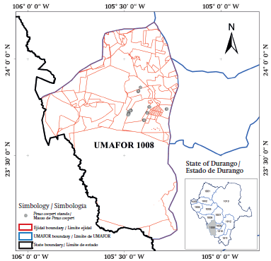
Figure 1 Location of the study area and location of the stands of Pinus cooperi analyzed for the development of a crown profile model.
Through field expeditions in the different ejidos of the UMAFOR 1008, P. cooperi were randomly sampled to measure their profile. Likewise, it was intended that the sampled trees corresponded to different combinations of site quality, age, density and sociological classes. i) Diameter at breast height (D, cm) recording two measures, one according to the direction north-south and the other east-west, using a caliper (Haglof, Sweden), with milimetric graduation; ii) total height (TH, m) from the ground to the apex of the tree using a hypsometer (Vertex IV®, Haglof, Sweden); iii) height of the base of the live crown (HBLC, m) measured to the interception of the first whorl with live needles on the trunk; iv) crown length (CL, m) obtained from the difference between TH and HBLC; and finally, v) maximum crown width (MCW, m) obtained from the average record of perpendicular directions (north-south and east-west) using a longimeter (Haglof, Sweden). Simultaneously, the main stand variables (density [trees∙ha-1], basal area [m2∙ha-1] and dominant height [m]), corresponding to sites where sample trees were collected, were also recorded.
Measuring crown profiles of P. cooperi
The area used by the projection of the crown is normally measured with the help of mirrors and tape measures; however, measuring the radius of the crown at different heights is a difficult task to perform (Gadow, Sánchez, & Álvarez, 2007). The crown profile of each tree was measured using a device developed by Hussein, Albert, and Gadow (2000). The device consists of a piece of transparent methacrylate (0.25 x 0.40 m) attached to a wooden stand which is fixed to the floor, so that the instrument remains stationary while measurements are taken. A transparency divided into squares of equal size, was overlapped on the methacrylate, which served as a reference to develop measurements. The device was located at a distance possible to fit the entire tree crown on the transparency. The characteristic points of the outer profile of the tree crown were drawn on the transparency, without moving the point-of-view or the crown window: i) top of the tree, ii) insertion of the first whorl with live pine needles on the trunk, iii) points where the first live pine needles are located and significant points of the outer edge of the tree crown. Figure 2 shows the variables of measured crowns and the geometric relationships used with this methodology.
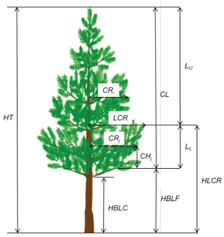
Figure 2 Scheme of crown variables of Pinus cooperi and geometric relationships between them. HBLC = Height of the base of the live crown; HBLF = Height of the first live needles; HLCR = height of maximum crown radius; CR = crown radius at each measurement point (i for the light crown, j for the shaded crown); CH = height of each crown radius from the base of the crown; LCR = maximum crown radius; CL = Total length of the crown; LU and LL = Length of the light crown and shaded crown, respectively; TH = Total height of the tree.
Visual methods have shown good accuracy in measuring crown radius and its corresponding height (Hussein et al., 2000; Rautiainen & Stenberg, 2005) and other crown variables (Martín-García, Diez, & Jactel, 2009).
Once known the length of tree crown (CL = TH - HBLC) and measured the distance between the top of the tree and the point of the crown base on transparency, the ratio CLreal/CLtransparency showed the scale used to calculate the radius of each point of the profile and its vertical distance from the crown base. After the crown profile was captured on the template, transparency was digitized by inserting the image in a CAD software and later obtaining the coordinates of each point of the crown profile using the “adxycoo.ave” script developed for the ArcView® software (Environmental Systems Research Institute [ESRI Inc.], 2002). Then, the image was aligned and scaled so that the points defined by the crown base (100, 0) and the top of the tree (100, CLreal) coincide with the vertical axis (the value of 100 was assigned to avoid negative numbers in the left profile of the crown). Figure 3 shows the coordinates of each point of the crown profile that led to the development of a spreadsheet to perform statistical adjustments.
Moreover, according to Maguire and Hann (1989), the height at which the first live needles occur (HBLF) was used as the crown base, discarding the insertion point of branch whorl (HBLF). This also dismiss the problem of finding lower values of HBLF than HBLC, because if the latter value is used as a start reference of the crown, the radii of the crown should be measured below the origin and consequently heights would be negative (Crecente-Campo, Álvarez-González, Castedo-Dorado, Gómez-García, & Diéguez-Aranda, 2013). Table 1 shows variables and descriptive statistics of the sample trees used to develop the equations of crown profile.
Table 1 Descriptive statistics of the sample trees used for fitting the models of the crown profile of Pinus cooperi.
| Statistics | Measurement points per crown | D (cm) | TH (m) | HBLC (m) | CL (m) | CR (m) |
|---|---|---|---|---|---|---|
| Average | 8.4 | 30.8 | 17.2 | 11.2 | 5.9 | 1.3 |
| Miminum | 6.0 | 9.7 | 6.5 | 1.6 | 1.6 | 0 |
| Maximum | 13.0 | 60.0 | 29.5 | 26.6 | 15.5 | 5.9 |
| Standard Deviation (±) | 1.35 | 13.8 | 5.7 | 5.4 | 2.3 | 1.1 |
D = Diameter at breast height; TH = Total height, HBLC = Height of the base of the crown, CL = Crown length, CR = Crown radius at each measurement point.
Models analyzed
Table 2 shows the models selected to describe the crown profile of P. cooperi. Among the models, we can found both simple geometric shapes that do not require adjustment (ellipsoids and cones) and more complex mathematical models.
Table 2 Models used to describe the crown profile of Pinus cooperi.
| Model | Mathematical expression |
|---|---|
| Ellipsoids | |
| Cone | |
| Polynomials | |
| Pretzsch (1992) | |
| Baldwin and Peterson (1997) modified | |
| Hann (1999) | |
| Rautiainen and Stenberg (2005) |
Where: CRi and CRj = Radius of the light Crown and shaded crown (m), respectively, at each measurement point; LCR = Light crown radius (m); Di and Dj: vertical distance between each radius of light crown and shaded crown, respectively, relative to the maximum crown radius (HLCR); Lu and Ll = length of the light crown and shaded crown (m), respectively; RCR = Relative crown radius (dimensionless); RCH = Relative crown height(dimensionless); z = Degree of the polynomial; TH = Total height (m); d = diameter at breast height (m); a0-az, b0-bz = parameters to be estimated in the adjustment.
Most models analyzed use two equations, one for estimating the light crown and another one to estimate the shaded crown. There are also models like polynomial models or the model of Baldwin and Peterson (1997), which with one formula estimate the entire crown. In this particular case, the model of Baldwin and Peterson (1997) was modified to include the variable crown maximum radius (LCR) in its formulation, following that proposed by Crecente-Campo, Marshall, LeMay and Diéguez-Aranda (2009). The models of Pretzsch (1992) and Hann (1999) have similar formulations although the latter includes the variables HT and D, making it more flexible than the first. In the case of the model of Hann (1999), the equation for the shaded crown (Table 2) has been previously used to model the profile of the shaded crown of P. radiata D. Don (Crecente- Campo et al., 2009), P. pinaster Ait. and P. sylvestris L. (Crecente-Campo et al., 2013). Finally, the model of Rautiainen and Stenberg (2005) has the drawback of only providing estimates for the light crown.
Fitting and selecting models
The parameters of linear models (polynomial) were estimated using the ordinary least squares method using the REG procedure of the SAS/STAT® package software (Statistical Analysis System [SAS Institute Inc.], 2004). The parameters related to the nonlinear models were estimated using an iterative procedure (Draper & Smith, 1981) which provides the smallest sum of squared errors using the Gauss-Newton algorithm (Hartley, 1961), implemented in the procedure MODEL of the SAS/ETS® statistical package (SAS, 2004). The goodness-of-fit of the models were analyzed from numerical comparisons of statistical coefficient of determination (R2) defined for Nonlinear regression (Ryan, 1997) and root mean square error (REMC) together with the visual inspection of scatterplots of residual versus predicted values of each one of the fitted models.
Results and discussion
Table 3 shows the parameter estimates and their standard errors for each model tested. It is noteworthy that all parameters were significant (P = 0.05), except for the parameter a1 of Hann’s model (1999), so the model was refitted without this parameter.
Table 3 Parameter estimates and standard errors of the models analyzed to predict the crown profile of Pinus cooperi (P = 0.05).
| Model | Parameter | Estimate | Standard error |
|---|---|---|---|
| Second-degree polynomial | a0 | 0.797 | 0.009 |
| a 1 | 1.400 | 0.046 | |
| a 2 | -2.152 | 0.044 | |
| Third-degree polynomial | a 0 | 0.820 | 0.009 |
| a 1 | 0.429 | 0.106 | |
| a 2 | 0.593 | 0.278 | |
| a 3 | -1.825 | 0.183 | |
| Fourth degree polynomial | a 0 | 0.812 | 0.008 |
| a 1 | 2.089 | 0.255 | |
| a 2 | -8.079 | 1.252 | |
| a 3 | 11.900 | 1.943 | |
| a 4 | -6.715 | 0.946 | |
| Fifth degree polynomial | a 0 | 0.816 | 0.008 |
| a 1 | -0.624 | 0.522 | |
| a 2 | 13.384 | 3.827 | |
| a 3 | -46.275 | 10.013 | |
| a 4 | 58.222 | 11.013 | |
| a 5 | -25.521 | 4.313 | |
| Pretzsch (1992) | a 1 | 0.326 | 0.014 |
| b 1 | 1.620 | 0.031 | |
| a 1 | 3.395 | 0.070 | |
| Baldwin and Peterson (1997) modified | a 2 | -4.164 | 0.064 |
| Hann (1999) | a 0 | 0.248 | 0.031 |
| a 2 | 0.149 | 0.059 | |
| b 1 | 0.737 | 0.007 | |
| b 2 | 0.604 | 0.147 | |
| Rautiainen and Stenberg (2005) | a 1 | 1.811 | 0.020 |
Table 4 shows the goodness-of-fit statistics of the models analyzed. The models that best described the light crown were the models of Pretzsch (1992), Hann (1999), and Rautiainen and Stenberg (2005) because they account for more than 98 % of the variability of the crown radius at different heights, with a lower value of REMC of 0.19 m. Moreover, the model of Hann (1999) had the best result in the adjustment of shaded crown because it accounts for 92 % of the variability of the sample, with a REMC value of 0.26 m. Finally, in the description of the profile of the entire crown, the model that showed the best results was also the model of Hann (1999), accounting for 96 % of the variability of the crown radius, with a REMC value of 0.21 m. Polynomial models provided good results, accounting for about 92 % of the variability of the crown radius, with a REMC of 0.29 m, improving the values of goodness-of-fit statistics as the degree of the polynomial increased.
Table 4 Statistical goodness-of-fit of the models used for predicting the crown profile of Pinus cooperi.
| Model | Total crown | Light crown | Shaded crown | |||
|---|---|---|---|---|---|---|
| R2 | REMC | R2 | REMC | R2 | REMC | |
| Two ellipsoids | 0.634 | 0.785 | 0.980 | 0.172 | 0.460 | 1.167 |
| Two cones | 0.583 | 0.923 | 0.854 | 0.529 | 0.426 | 1.256 |
| Ellipsoid-Cone | 0.467 | 0.824 | 0.980 | 0.172 | 0.426 | 1.256 |
| Cone-Ellipsoid | 0.549 | 0.902 | 0.854 | 0.529 | 0.460 | 1.167 |
| Combination ellipsoid-truncated cone | 0.883 | 0.384 | 0.980 | 0.172 | 0.655 | 0.548 |
| Second-degree polynomial | 0.918 | 0.317 | 0.926 | 0.272 | 0.862 | 0.366 |
| Third-degree polynomial | 0.927 | 0.298 | 0.943 | 0.238 | 0.857 | 0.373 |
| Fourth degree polynomial | 0.935 | 0.283 | 0.955 | 0.213 | 0.863 | 0.365 |
| Fifth degree polynomial | 0.938 | 0.277 | 0.961 | 0.196 | 0.861 | 0.368 |
| Pretzsch (1992) | 0.887 | 0.371 | 0.983 | 0.149 | 0.659 | 0.538 |
| Baldwin and Peterson (1997) modified | 0.896 | 0.367 | 0.918 | 0.345 | 0.859 | 0.359 |
| Hann (1999) | 0.962 | 0.214 | 0.984 | 0.147 | 0.921 | 0.259 |
| Rautiainen and Stenberg (2005) | 0.981 | 0.183 | ||||
REMC: Root mean square error. Models based on ellipsoids and two cones did not provide satisfactory results for the shaded crown because they are defined to be equal to 0 at the beginning of the crown.
Figures 4, 5 and 6 show scatterplots of residual against predicted values for the radii of the entire crown, light crown and shaded crown of each of the models tested. The models of Baldwin and Peterson (1997), Hann (1999) and Rautiainen and Stenberg (2005), and the polynomial models showed a good residual distribution; in contrast, the ellipsoid and the cone did not show such distribution.
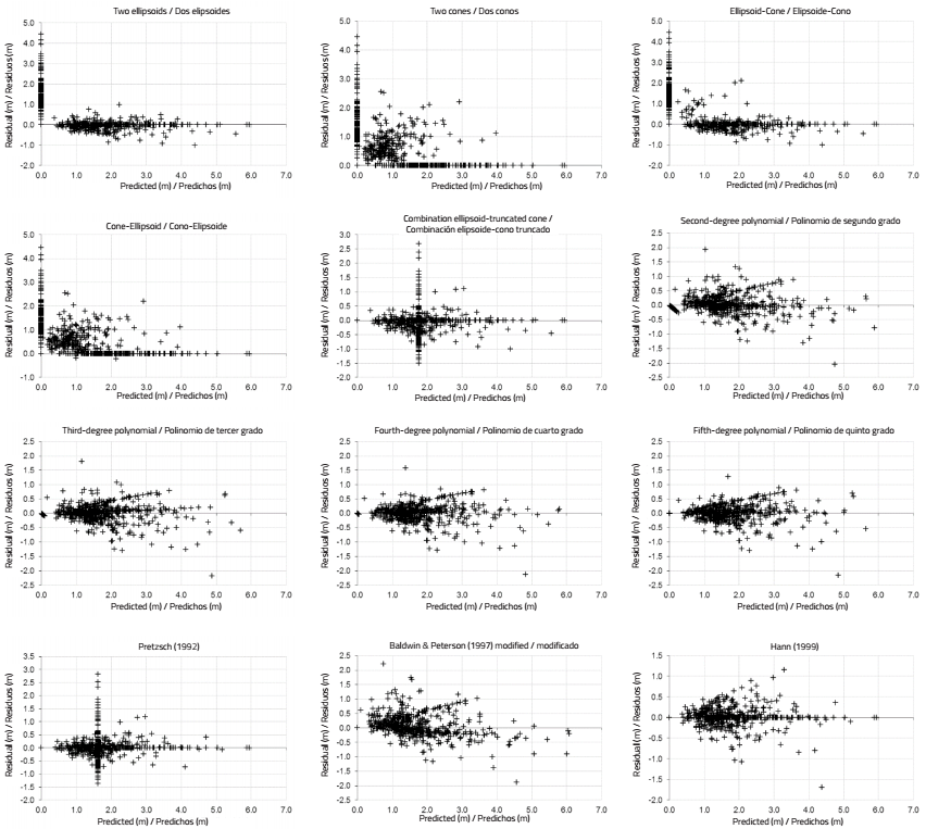
Figure 4 Scatterplots of residual against predicted values describing the entire crown radius of Pinus cooperi.
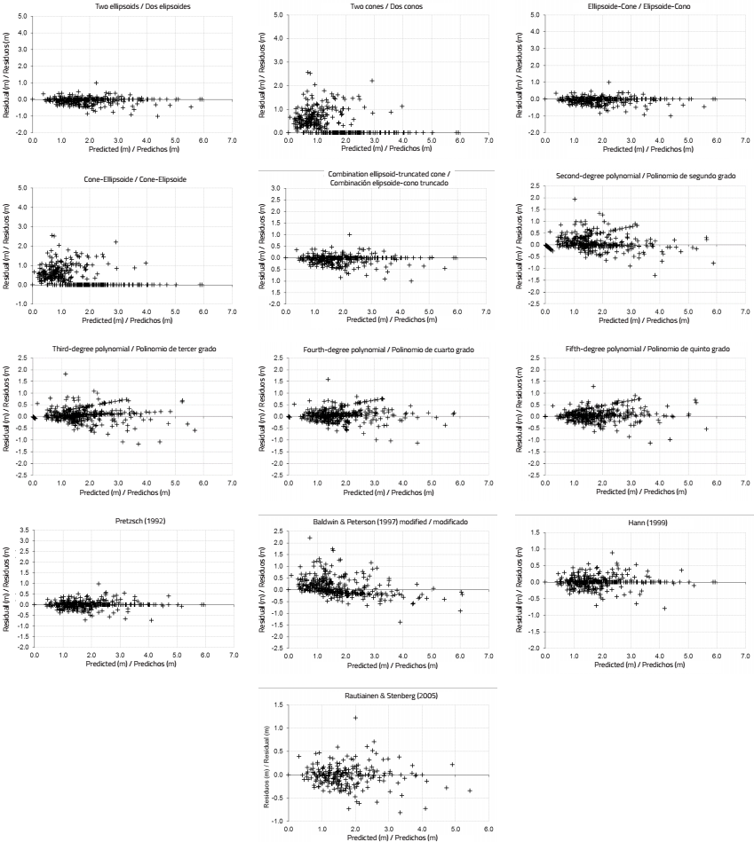
Figure 5 Scatterplots of residual against predicted values describing the light crown radius of Pinus cooperi.
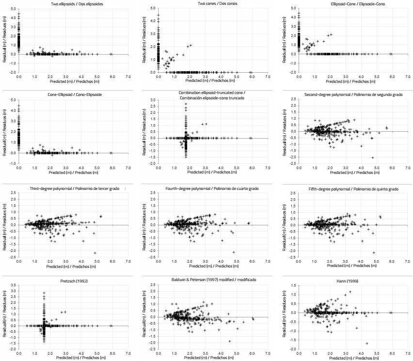
Figure 6 Scatterplots of residual against predicted values describing the shaded crown radius of Pinus cooperi.
A criterion that could be used to choose the best model to describe the crown profile is the number of variables required. In this sense, the model that includes more variables is that less useful because it also increases the time and cost of inventory. Following this approach, the best models are the polynomial, as for application only require the full crown length and its maximum radius. All other models analyzed need three variables (total length and maximum crown radius, and distance from the maximum radius to the base of the tree).
Since the current height measuring devices do not require to be placed at a known distance from the tree, to take height measurements at which the maximum crown radius is reached is fast; therefore, in the case of having this kind of devices, it is advised to use the model of Hann (1999) for estimating the crown profile of P. cooperi in the study area. The model proposed has the advantage that varies the profile by including the slenderness ratio (HT/D) into the equation of light crown. For example, trees that grow in denser stands will have higher coefficients of slenderness (taller and thinner trees), so the exponent of the model will be higher and the light crown will be more conical, while in the case of less dense stands, light crowns will be more parabolic. The social status of the tree also affects the shape of the crown so that the dominant trees with smaller slenderness will have more parabolic light crowns compared to trees of the lower strata. This coefficient has also been included in the crown models of other species such as Pseudotsuga menziesii (Mirb.) Franco in Oregon’s Forests (Hann, 1999) or in pure and even-aged stands of P. radiata in the northwest of Spain (Crecente-Campo et al., 2009). Stand age is not part of the model, however, it indirectly affects the shape of the light crown and shaded crown as the length of the crown, the maximum radius and the height at which this is achieved varies with age.
Conclusions
The system of equations developed from the model of Hann (1999), which includes a model for the light crown and other for the shaded crown, provided accurate estimates for both the entire crown and light crown and shaded crown of P. cooperi in UMAFOR 1008 (El Salto, Pueblo Nuevo, Durango). With this model it will be possible to develop competition indices to help in the selection of trees to be removed for thinning in order to optimize the individual tree growth. The results provide support silvicultural tools in data collection protocols, and to optimize the resources needed for fieldwork and further development of the set of equations of a dynamic stand model for the species studied.


 texto en


