Introduction
Mexico has a land area of about 1 959 million km2, where topography has given many watersheds, ranging in size from 200 to 20 000 km2. However, it only has 815 operational hydrometric stations (National Water Commission [CONAGUA], 2019), which makes it impossible to monitor runoff volumes in all watersheds, especially in those that are difficult to access.
Having records of river and stream flow is crucial for understanding water availability, its temporal and spatial variations, and its utilization in the planning, management, operation, and design of projects related to surface water (World Meteorological Organization [WMO], 2010). When actual runoff data is lacking, reliance is placed on the inference through hydrological models. However, these models, developed in other parts of the world, may not be suitable due to variations in how basins respond to precipitation (Gupta et al., 2008; Hrachowitz et al., 2013).
Although there is currently abundant research focused on the precise quantification of water volumes, especially concerning the design of flow meters for water measurement in the agricultural sector, most studies have been conducted with clean water (Replogle, 1970; Replogle & Clemmens, 1981; Clemmens et al., 1984; Clemmens et al., 1987; Bos, 1989; Clemmens & Bos, 1992; Clemmens et al., 2001; Cox et al., 2013). There is a smaller proportion of research on flume for sediment-laden flow (Wilm et al., 1938; Gwinn, 1964; Smith et al., 1981; Göğüş & Altinbilek, 1994; Castro-Orgaz & Mateos, 2014).
Thanks to the conducted research, Wahl et al. (1999) developed WinFlume®, a computer program that facilitates the design and calibration of long-throated flumes and broad-crested weirs for flow measurement, with errors of approximately 2 %, as detailed by Clemmens et al. (2001). Traditionally, measurements are taken through a stilling well located in the inlet section of the structure; however, sediment transport promotes blockage of the entry conduits to the measurement wells, hindering measurements and resulting in the loss of temporal flow evolution. To address this issue, Replogle suggested adding a steeper slope to long-throated flumes in natural basins and installing an additional stilling well in this section. Thus, flow measurements during the rising limb of the hydrograph can be taken in the original well, and when it fails due to sediment accumulation, information can be complemented with data collected from the well located in the steeper slope (Wahl et al., 2000).
The WinFlume® program does not include hydraulic analysis in the steeper slope, so it is necessary to turn to other programs to analyze the hydraulic behavior in this area in order to determine the optimal location for measurements. Thanks to research in hydraulic structures and advances in computing, several programs related to Computational Fluid Dynamics (CFD) are now available. These programs are capable of numerically simulating the behavior that the water flow will exhibit through various geometric shapes of hydraulic structures (Bermúdez et al., 2017; Bladé et al., 2019; Carrillo et al., 2018; Echeverribar et al., 2019; Hafnaoui & Debabeche, 2020; Zeng et al., 2019).
This research is based on a previous analysis of flumes with different geometries, which resulted in the proposal of a rectangular section long throat flume with a steeper slope. Based on the above, the objective of the present study was to analyze the hydraulic behavior of a long-throat flume with modification, to locate the optimum site for taking readings when there are excess sediments, by means of 1D numerical simulations (HEC-RAS® V. 5.06), 2D (Iber® V. 2.5.2) and 3D (ANSYS® CFX® V. 2020 R2).
Materials and methods
An acrylic (polymethylmethacrylate) long-throat flume, with absolute roughness ks of 0.00006 m, was designed using WinFlume® v.1.06 software for a maximum flow rate of 50 L∙s-1. The flow rate vs. flow depth curve (Q vs. h) of the flume, a flume table for circulating flow rates in a range from 2 to 50 L∙s-1 (measured with depths in 1 cm increments, 22 flow rates) and its corresponding curve fitting equation were obtained. To this structure, a steeper slope with the same dimensions of the throat was added, considering four slopes in supercritical regime.
Geometric model for clean water
The flume structure, along with the proposed modifications, consists of:
A rectangular approach channel, 0.5 m in length, with a bottom slope of zero, a base width of 0.40 m, and a depth of 0.40 m.
A converging transition section, 0.3 m in length, centered on the axis, gradually rising 0.05 m above the bottom of the approach channel. Downstream of this section, the resulting dimensions are 0.25 m base and 0.35 m depth.
A rectangular control section (throat) of 0.35 m in length, with a bottom slope of zero, 0.25 m width and 0.35 m depth.
A weir that maintains the dimensions of the control section; in other words, a rectangular channel with a base width of 0.25 m and a depth of 0.35 m. Its horizontally measured length is 0.5 m, and it has a variable outlet level.
Since the steeper slope is the area of interest, four different structures were configured corresponding to slopes of 30, 20, 10, and 5 %. Figure 1 shows the geometry of the flume for a steeper slope with a 30 % slope.
Due to the need to use a Manning's n coefficient in 1D and 2D simulations, a conversion was performed using an equation derived from Manning's and Darcy-Weisbach's (Equation 1) and Colebrook's (Equation 2) expressions:
where n is the Manning's roughness coefficient (dimensionless), g is the acceleration of gravity (m∙s-2), R h is the hydraulic radius (m), f is the Darcy friction factor (dimensionless), k is the absolute roughness (m), D is the hydraulic diameter (m) and Re is the Reynolds number (dimensionless)
For the conversion, information from the flume table generated with WinFlume® was used, where, based on the various depths and flow velocities corresponding to each discharge, as well as the geometric properties of the structure, a Manning's n value was calculated, to finally obtain the average value that resulted in 0.0123.
Geometric model of the sediment-modified flume system
Four structures, similar to those designed for clean water, were used. However, there was a reduction in hydraulic area in both the approach channel and the converging transition section, affecting them at the bottom. This is because sediment accumulation at the bottom of the flume is anticipated, aligning with the throat or control section's bottom. Figure 2 shows the reduced zone, using a structure as an example.
The resulting structure exhibits a zero slope in the initial three sections, with the new transition section featuring only a gradual constriction of the walls. As the reduction in hydraulic area in the two sections preceding the throat is presumed to be caused by sediment accumulation, a Manning's coefficient of 0.023 was suggested exclusively for the bottom, taking into account the characteristics of the deposited material (Chow, 1988). The Manning's coefficient of 0.0123 was maintained for the other walls.
Hydraulic simulations
To characterize the hydraulic behavior of the proposed structure, three approaches were considered: one-dimensional, two-dimensional, and three-dimensional. Simulations of the flume structure with the geometric model for clean water were conducted using all three approaches. However, the sediment-modified structure was only used in two-dimensional simulations due to the computational cost associated with three-dimensional analysis. It was a balance to avoid oversimplifying the analysis to the one-dimensional approach.
In all cases, simulations were performed for each discharge obtained from the flume table created during the design with WinFlume v.1.0.6. In total, 88 discharge simulations were conducted with HEC-RAS® (four slopes), 176 simulations with Iber® (four slopes and two scenarios), and 88 simulations with ANSYS® CFX® (four slopes).
One-dimensional simulation
This simulation was conducted using the HEC-RAS® v.5.0.7 program, which is based on solving the Saint-Venant equations, assuming that water flow occurs only in the longitudinal direction of the hydraulic structure, represented by cross-sectional profiles. The program has the capability to calculate water surface profiles for steady and gradually varied flow in natural or artificial channels, considering subcritical, supercritical, and mixed flow regimes (Brunner, 2016). For steady flow, water surface profiles are calculated using the energy equation between cross-sectional profiles (Equation 3) through an iterative procedure (Brunner, 2016):
where Z 1 and Z 2 are the elevation of the channel bottom, Y 1 and Y 2 re the water depth, V 1 and V 2 are the mean flow velocities, ( 1 and ( 1 are the velocity weighting coefficients, g is the gravitational acceleration, and h e is the energy loss.
The geometric model was generated using cross sections every 10 cm at the inlet, throat and steeper slope, and sections every 5 cm in the convergence zone, with a Manning's coefficient of 0.0123 on the walls of each simulated structure.
The imposed boundary conditions at de begin of simulation, were normal depth at the inlet of the structure and critical depth at the outlet. In the first case, a bed slope of 1×10⁻⁶ m was established to avoid indeterminacies in the numerical calculation of hydraulic profiles, as HEC-RAS® uses the Manning equation with the user-introduced friction slope (S f ), which takes the form Q = K(S f ) 0.5 . Flow rates were simulated in a steady-state under mixed flow regime.
Two-dimensional simulation
The two-dimensional simulation was conducted using Iber® v.2.5.2, which solves the Saint Venant equations by the finite volume method. These equations represent the principles of conservation of energy and momentum for a moving volume of water, while also accounting for the effects of turbulence and friction caused by the wind on the water surface (Bladé et al., 2014):
where h is depth, U x and U y are the horizontal velocities in the main and transverse directions of the flow averaged in depth. g is acceleration due to gravity, ρ is water density, Z b is the bottom elevation, ( s is the friction at the free surface due to friction caused by the wind, ( s is the friction due to bottom friction, and v t is turbulent viscosity. Bottom friction in the channel is calculated using the Manning equation in the main and transverse directions of the flow:
The friction on the free water surface caused by the wind is calculated using the Van Dorn equation, considering the wind speed at 10 m above the free water surface (Van Dorn, 1954).
The geometric models originally proposed for clean water (Figure 1) and modified by sediments (Figure 2) were configured, with Manning coefficients assigned as 0.0123 on the walls of the structures, except at the bottom of the inlet channel and the convergent transition section of the models modified by sediments, where the value of n was 0.023. The numerical discretization consisted of a structured mesh with rectangular elements of 0.5 cm × 1.0 cm, with the longer side in the main flow direction.
The boundary conditions at the inlet were constant flow under subcritical regime, and supercritical regime flow at the outlet. Furthermore, the k-( turbulence model of Rastogi and Rodi (1978) was defined.
Three-dimensional simulation
This simulation was conducted using the academic version of ANSYS® CFX® v.2020 R2, a Computational Fluid Dynamics (CFD) program that integrates advanced numerical solutions for the general equations of fluid flow with powerful preprocessing and postprocessing capabilities. Additionally, it can model laminar and turbulent flows in steady-state or transient conditions. This program employs the finite volume method to discretize the problem domain and solve the Reynolds-averaged Navier-Stokes (RANS) differential equations for each control volume (ANSYS, 2020).
The equations for the conservation of mass and momentum can be expressed as follows:
where i and j are indexes representing
directions, where x
i
denotes the coordinate directions (i = 1 to 3 for
x, y, z directions),
( is the density of the flow, t is
time, U is the velocity vector, p is
pressure, u’
i
represents turbulent velocity in each direction (i =
1 a 3 for x, y, z
directions), μ is molecular viscosity, S
ij
is the mean rate-of-strain tensor, and -(
The model geometry was prepared using the SALOME® v.9.5.0 software (Open Cascade, 2021). Subsequently, it was imported into ANSYS® CFX®, where the domain discretization was performed using a “multizone” meshing method, generating approximately 300 thousand hexahedral elements. The maximum side length of the elements was set to 1 cm, ensuring good asymmetry parameters (max. 0.156) and orthogonal quality (min. 0.96). These parameters are crucial for any simulation (ANSYS, 2020).
The simulation was conducted under steady-state conditions at a pressure of 1 atm, using water and air as incompressible fluids. The homogeneous Eulerian-Eulerian multiphase flow model was selected to solve the two-phase air-water flow, and a free surface model was chosen for the interface. The surface tension model was defined as a continuous surface force with water as the primary fluid, using a surface tension coefficient of 0.072 N·m-1 and the standard k-( turbulence model. The boundary conditions included fluid velocity at the inlet of the control volume, fluid outlet at static mean pressure, the top of the open structure at atmospheric pressure, and the walls of the structure treated as immovable with a roughness of 0.00006 m.
Measurement and processing of results
Six water depth measurement sites were selected: one at 0.2 m from the inlet of the structure (site E) and five in the steeper slope (distributed equidistantly from the start) (Figure 3). For both 2D and 3D simulations, measurements were taken at up to seven points across the structure to obtain an average value.
To determine the reliability of the obtained results, three types of errors were calculated at each measurement site: mean absolute percentage error (MAPE), root mean square error (RMSE), and mean absolute error (MAE) (Khuntia et al., 2019; Sammen et al., 2020), using the following equations:
where ( iobs is the value predicted with WinFlume, ( i is the value obtained from the hydraulic simulation (1D, 2D and 3D) and N is the number of data analyzed.
The Q vs. h curves obtained with WinFlume® and from the simulations were plotted together in order to visualize the variation between them. Subsequently, with the flow depth values measured at each site selected in the steeper slope for the simulated flow rates, flow profile plots were constructed, in order to identify the site showing the greatest consistency in the variation of the flow lines, since the flow rates were defined for fixed flow depth increments.
On the other hand, in order to check whether the reduction of the hydraulic area at the flume inlet has an effect on the flow of the rapid, the errors described in Equations 10 to 12 were calculated for the results obtained in the simulations performed with the sediment-modified geometric models. For this purpose, the reference values obtained in the steeper slopes of the geometric models for clean water were considered.
Finally, the two measurement sites with the lowest error were selected to construct Q vs. h plots and obtain the fitting parameters of a potential model of the form Q = k·hm, as well as the coefficient of determination (R2), which expresses the fit of the model to the variable to be explained (Chicco et al., 2021).
Results and discussion
Table 1 shows the flow rates determined with WinFlume® for the proposed flow measurement structure (measured at the inlet), and Figure 4 shows typical Q vs. h curve of the structure.
Table 1 Important hydraulic variables determined at the inlet of the proposed flume system.
| Flow depth (h, cm) | Flow rate (Q, L∙s-1) | Froude number (Fr) | Velocity (m∙s-1) |
|---|---|---|---|
| 3.0 | 2.12441 | 0.07495 | 0.06639 |
| 4.0 | 3.33120 | 0.09850 | 0.09253 |
| 5.0 | 4.71405 | 0.11901 | 0.11785 |
| 6.0 | 6.25570 | 0.13689 | 0.14217 |
| 7.0 | 7.94286 | 0.15255 | 0.16548 |
| 8.0 | 9.76558 | 0.16633 | 0.18780 |
| 9.0 | 11.71547 | 0.17855 | 0.20920 |
| 10.0 | 13.78554 | 0.18944 | 0.22976 |
| 11.0 | 15.96933 | 0.19921 | 0.24952 |
| 12.0 | 18.26243 | 0.20801 | 0.26857 |
| 13.0 | 20.66366 | 0.21602 | 0.28700 |
| 14.0 | 23.16658 | 0.22332 | 0.30482 |
| 15.0 | 25.76660 | 0.22999 | 0.32208 |
| 16.0 | 28.45768 | 0.23608 | 0.33878 |
| 17.0 | 31.24218 | 0.24171 | 0.35502 |
| 18.0 | 34.11957 | 0.24695 | 0.37086 |
| 19.0 | 37.07784 | 0.25176 | 0.38623 |
| 20.0 | 40.09573 | 0.25608 | 0.40096 |
| 21.0 | 43.18549 | 0.26006 | 0.41525 |
| 22.0 | 46.37358 | 0.26389 | 0.42938 |
| 23.0 | 49.63846 | 0.26747 | 0.44320 |
| 24.0 | 52.97837 | 0.27083 | 0.45671 |
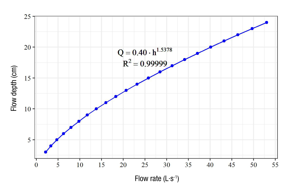
Figure 4 The relationship between flow rates (Q) and flow depth (h) calculated at the inlet of the proposed flume structure.
Figure 5 shows the results of simulations conducted with the three programs for a specific flow rate and slope. Table 2 shows the calculated errors of the hydraulic simulation results in comparison to those predicted by the WinFlume® program, revealing no significant differences. This aligns with the findings of Glock et al. (2019), who reported no substantial differences in water depths calculated using 1D, 2D, and 3D numerical models. Their study involved simulations of channels with varying morphologies and flow conditions, but without abrupt changes.
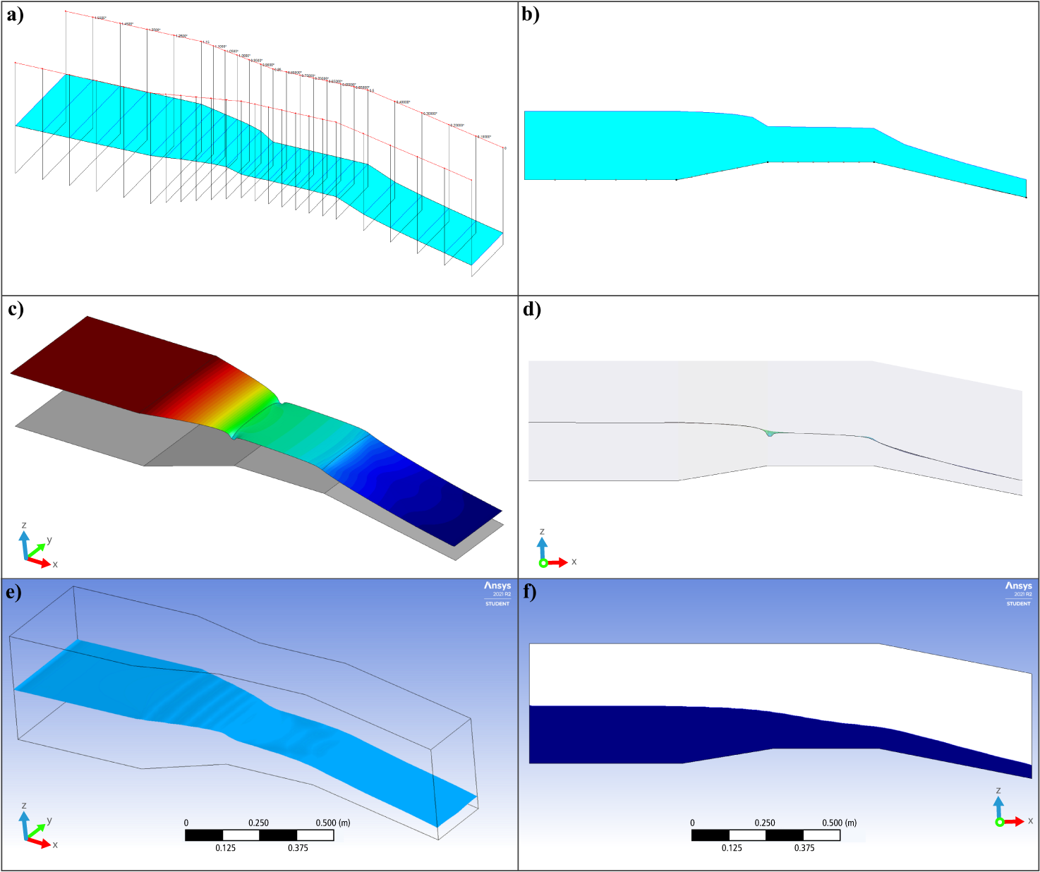
Figure 5 Flow behavior in a flume structure with a 20% downstream slope for a flow rate of 23.1666 L∙s-1: a and b) HEC-RAS®, c and d) Iber®, and e and f) ANSYS CFX®.
Table 2 Statistics determined for the results of the hydraulic simulations at the inlet of the structure.
| Program | Errors at the inlet of the structure | ||
|---|---|---|---|
| MAPE (%) | MAE (cm) | RMSE (cm) | |
| HEC-RAS (1D) | 2.28 | 0.015 | 0.371 |
| IBER (2D) | 2.73 | 0.018 | 0.471 |
| ANSYS CFX (3D) | 1.80 | 0.011 | 0.274 |
MAPE: mean absolute percentage error; MAE: mean absolute error; RMSE: root mean square error.
It is observed that the results obtained with all three programs had a good fit, as all errors are close to 0. This is also evident in the Q vs. h curves (Figure 6).
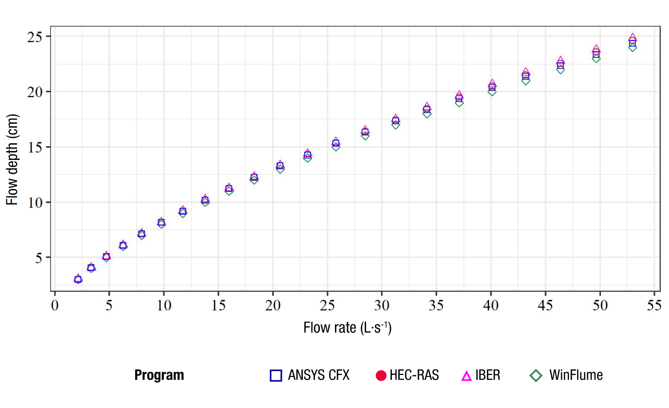
Figure 6 Comparison of water flow depth (h) calculated for different simulated flow rates (Q) at the inlet of the flume structure.
The results of the water flow profile behavior generated from the simulated flow rates are shown in Figures 7, 8, and 9. Overall, it is observed that the variation obtained between profiles is consistent; that is, for each simulated discharge, there is a fixed increase in flow depth. However, there are some locations where some data points do not conform to the expected normal behavior.
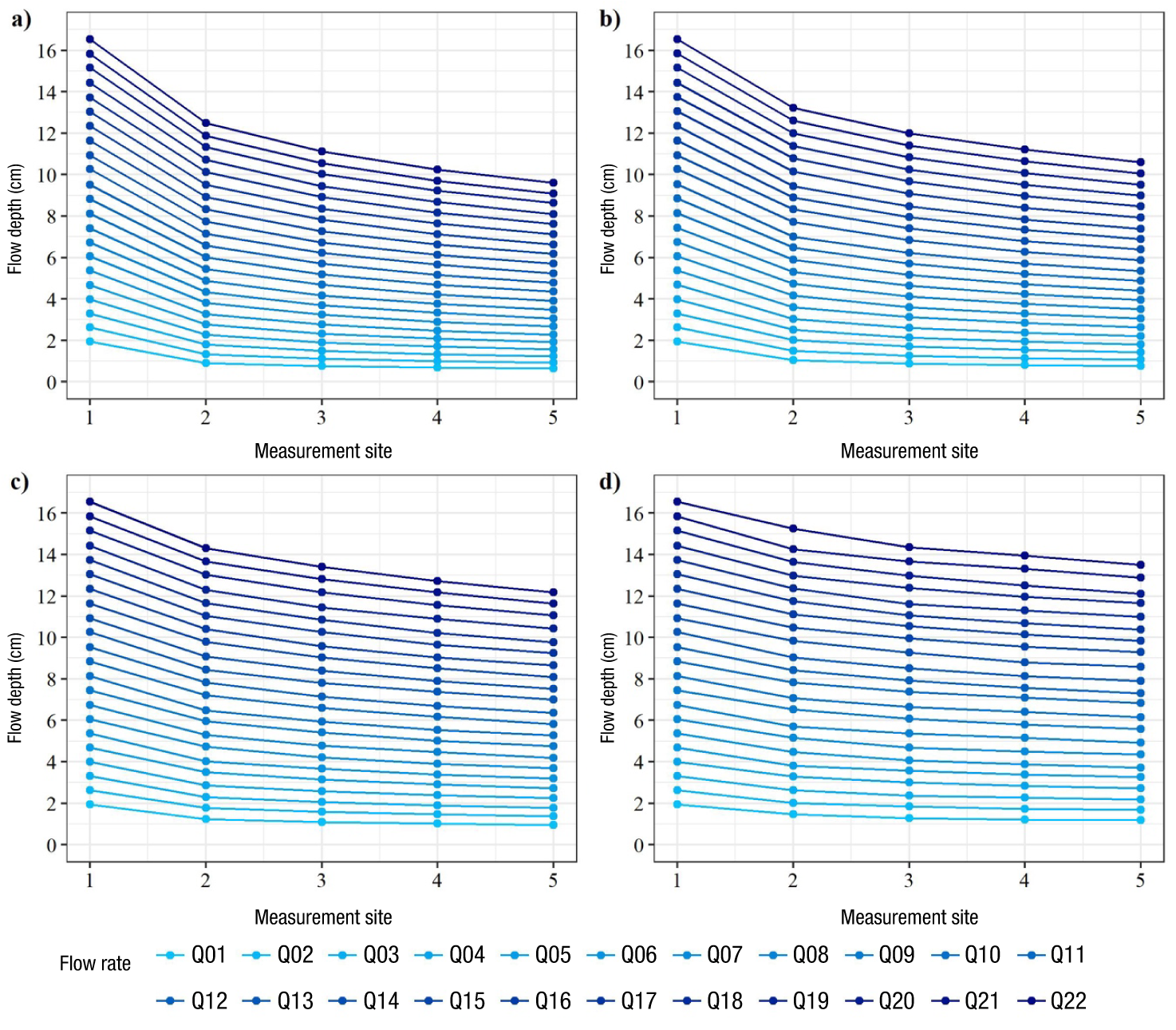
Figure 7 Water flow profiles obtained from the simulated flow rates using the HEC-RAS® program in the steeper slope of the flume structure with the evaluated slopes: a) 30 %, b) 20 %, c) 10 %, and d) 5 %.
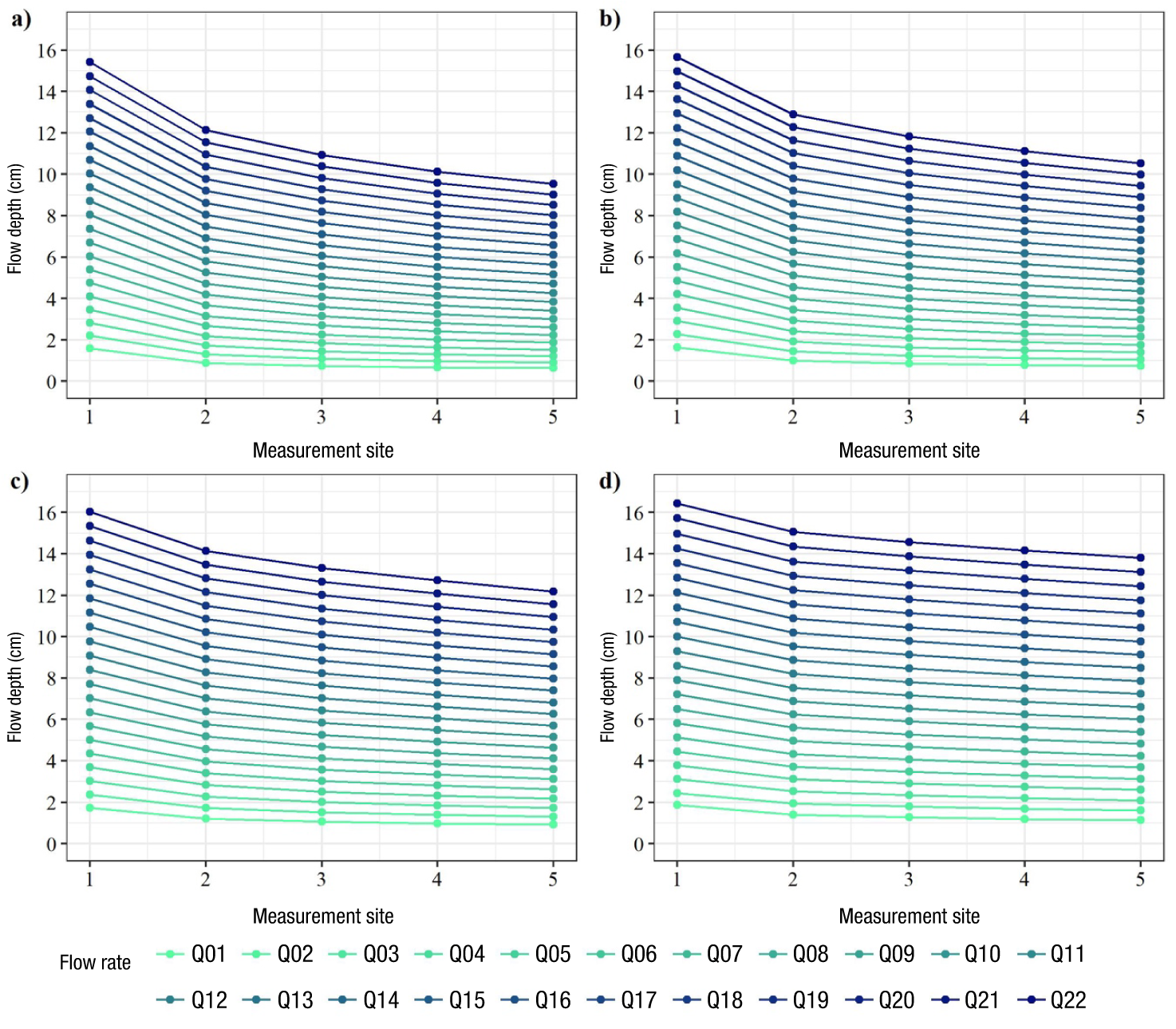
Figure 8 Water flow profiles obtained from the simulated flow rates using the Iber® program in the steeper slope of the flume structure with the evaluated slopes: a) 30 %, b) 20 %, c) 10 %, and d) 5 %.
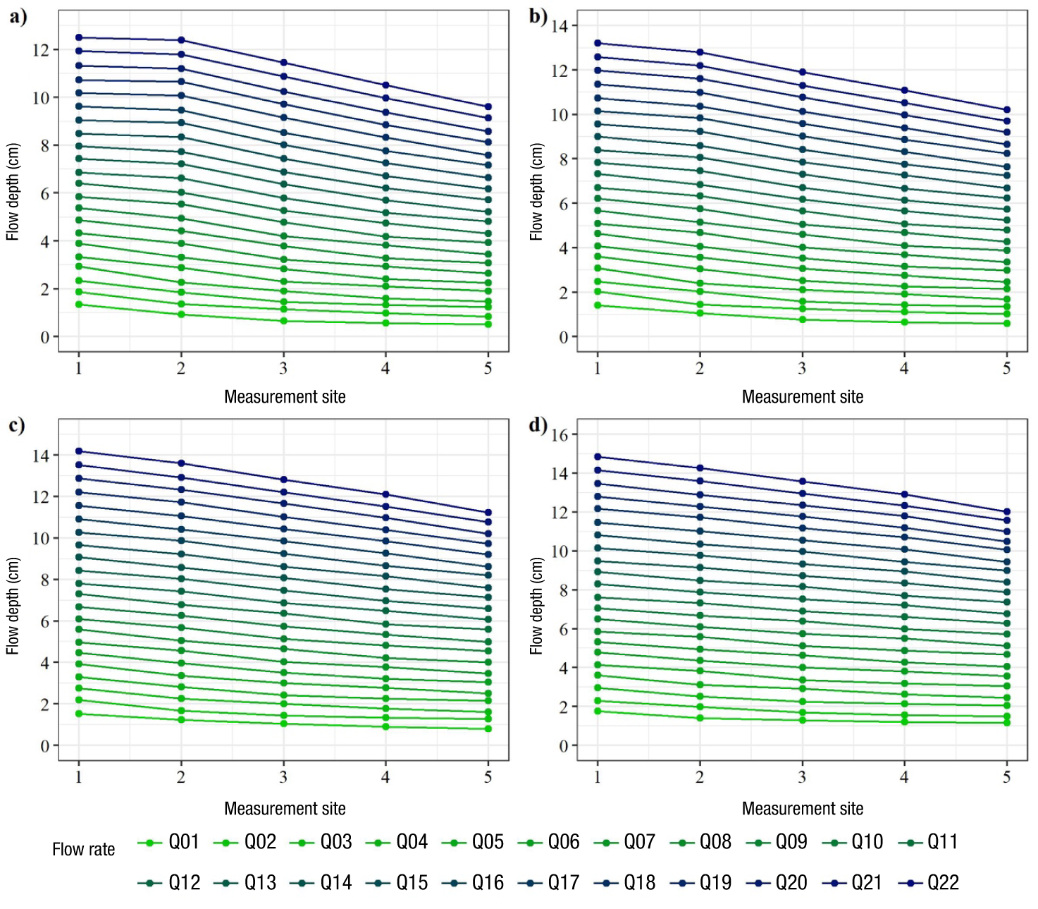
Figure 9 Water flow profiles obtained from the simulated flow rates using the ANSYS® program in the steeper slope of the flume structure with the evaluated slopes: a) 30 %, b) 20 %, c) 10 %, and d) 5 %.
Significant variation is observed in the graphs among the simulations. In the first site, the 1D simulation results (Figure 7) indicate the same value for a given flow rate, despite having a different downstream slope. However, in the 2D and 3D simulations (Figures 8 and 9, respectively), the value decreases as the downstream slope increases. This situation is similar to that described by Toombes and Chanson (2011), who analyzed flow using a physical model and 1D, 2D, and 3D simulations in a broad-crested weir with a curved downstream termination allowing flow acceleration. These authors concluded that, at regime transition sites, HEC-RAS® provides a higher depth value than what occurs, and this error increases with increasing flow rate.
In this research, it is important to highlight that inconsistencies were found among the flow profiles in the 3D simulations (Figure 9). A pattern was expected in the separation of the flow lines. These inconsistencies are evident at flow rates lower than 10 L∙s⁻¹ in the second sampling site with the four evaluated slopes. This could be attributed to the formation of waves caused by the reflection of convergent flow on the sidewalls of the flume structure (oblique jump). This corresponds to that reported by Krüger and Rutschmann (2006) and Abdo et al. (2018) in similar designs with supercritical flows.
Regarding the analysis of the flow profiles obtained from the simulations, it was found that the ideal sites for measuring flow depth and estimating flow rate through a functional relationship Q vs. h are sampling sites three and four. Although good agreement was also observed at site five, it could be influenced by flow conditions generated downstream of the structure. On the other hand, the analysis conducted to determine if the reduction of hydraulic area, caused by sediment accumulation at the inlet of the structure, influences flow depths in the steeper slope for different simulated flow rates is shown in Table 3
Table 3 Errors in flow depth between simulations in the steeper slope of the original flume structure and the flume structure with reduced hydraulic area
| Measurement site | Error | Slope of the steeper slope | |||
|---|---|---|---|---|---|
| 30 % | 20 % | 10 % | 5 % | ||
| 1 | MAPE (%) | 0.290 | 0.160 | 0.110 | 0.320 |
| MAE (cm) | 0.063 | 0.014 | 0.011 | 0.020 | |
| RMSE (cm) | 0.026 | 0.012 | 0.009 | 0.013 | |
| 2 | MAPE (%) | 0.090 | 0.100 | 0.120 | 0.220 |
| MAE (cm) | 0.009 | 0.010 | 0.016 | 0.025 | |
| RMSE (cm) | 0.007 | 0.007 | 0.012 | 0.019 | |
| 3 | MAPE (%) | 0.090 | 0.090 | 0.120 | 0.220 |
| MAE (cm) | 0.007 | 0.008 | 0.015 | 0.031 | |
| RMSE (cm) | 0.005 | 0.006 | 0.011 | 0.021 | |
| 4 | MAPE (%) | 0.110 | 0.080 | 0.140 | 0.220 |
| MAE (cm) | 0.006 | 0.008 | 0.016 | 0.032 | |
| RMSE (cm) | 0.005 | 0.005 | 0.011 | 0.022 | |
| 5 | MAPE (%) | 0.110 | 0.090 | 0.130 | 0.240 |
| MAE (cm) | 0.006 | 0.008 | 0.015 | 0.032 | |
| RMSE (cm) | 0.004 | 0.006 | 0.011 | 0.022 | |
MAPE: mean absolute percentage error; MAE: mean absolute error; RMSE: root mean square error.
The results in Table 3 confirm that the sites with the least variation in flow profiles are sites three, four and five, which would be suitable for measuring flow depth with greater reliability. The graphs of Q vs. h relationships derived from the 1D, 2D and 3D simulations at measurement sites three and four are shown in Figures 10 and 11, respectively.
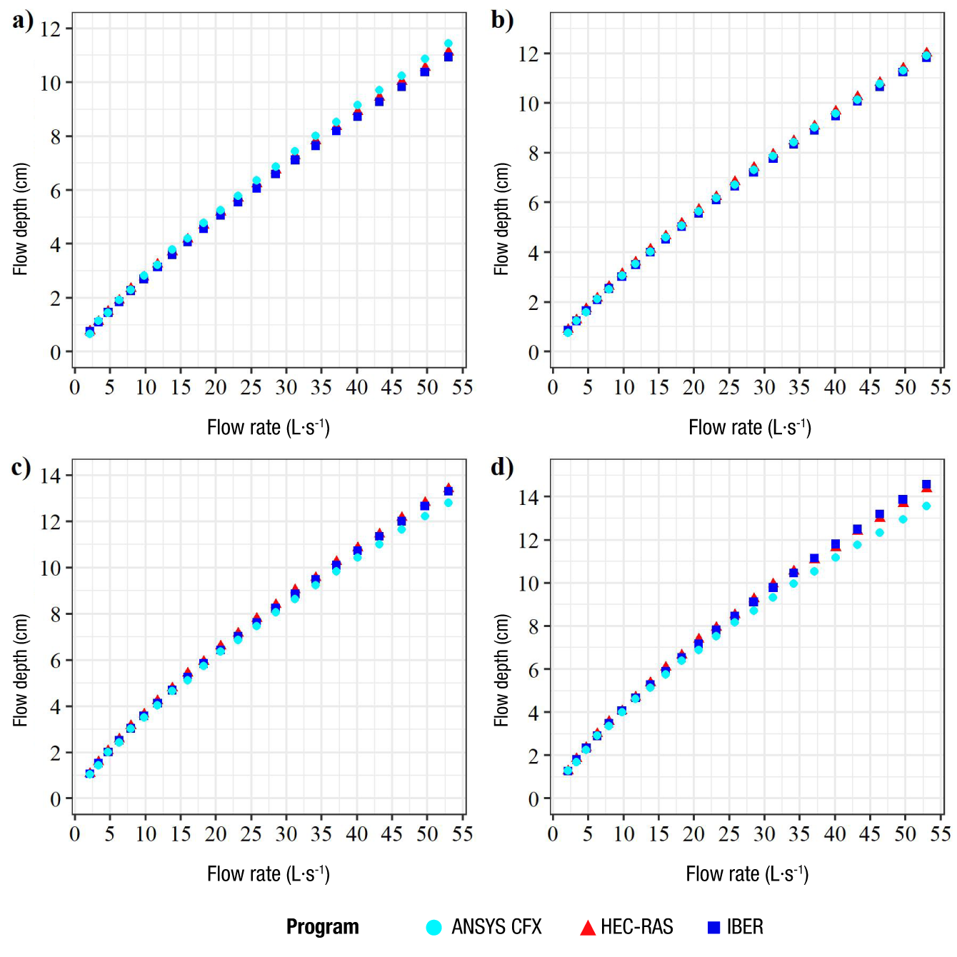
Figure 10 Comparison of flow rate (Q) vs. flow depth (h) relationships obtained at sampling site three in the proposed flume structure and with slopes in the steeper slope: a) 30 %, b) 20 %, c)10 % and d) 5 %.
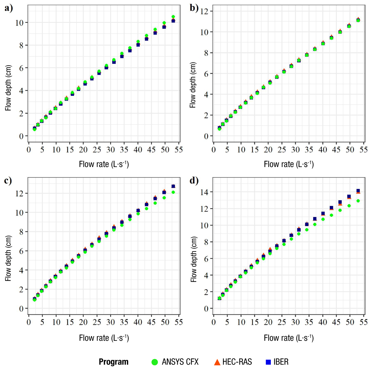
Figure 11 Comparison of flow rate (Q) vs. flow depth (h) relationships obtained at sampling site three in the proposed flume structure and with slopes in the steeper slope: a) 30 %, b) 20 %, c)10 % and d) 5 %.
Finally, Table 4 presents the results obtained at measurement sites three and four, fitted to the model of the form Q = k·hm, with their respective R2. In all cases, there is a high coefficient of determination, which means that there is a strong correlation between flow rates and flow depth. Toombes and Chanson (2011) mention that the results obtained with 3D simulations are of greater importance. In this case, it is observed that with the two major slopes, measurement site four had the best fit, while for the minor slopes there is a better fit at site three. However, it should be considered that the higher the slope, the smaller the variation between flow profiles, which would make their measurement more difficult, since precise instruments would be required. Therefore, it is advisable to use the lower slopes.
Table 4 Potential equation of flow rate (Q) vs. flow depth (h) relationship of sites three and four in the steeper slope of the flume structure for simulations 1D (HEC-RAS®), 2D (Iber®) and 3D (ANSYS® CFX®).
| S | M | HEC-RAS® | IBER® | ANSYS CFX® | |||
|---|---|---|---|---|---|---|---|
| Equation | R2 | Equation | R2 | Equation | R2 | ||
| 30 % | 3 | Q = 2.7692∙h1.2231 | 0.99992 | Q = 2.9065∙h1.2120 | 0.99996 | Q = 2.8059∙h1.2035 | 0.99984 |
| 4 | Q = 3.2470∙h1.1983 | 0.99996 | Q = 3.4310∙h1.1813 | 0.99999 | Q = 3.3906∙h1.1673 | 0.99985 | |
| 20 % | 3 | Q = 2.3117∙h1.2587 | 0.99992 | Q = 2.4653∙h1.2405 | 0.99997 | Q = 2.4210∙h1.2431 | 0.99983 |
| 4 | Q = 2.7168∙h1.2279 | 0.99997 | Q = 2.8334∙h1.2145 | 0.99997 | Q = 2.8650∙h1.2106 | 0.99985 | |
| 10 % | 3 | Q = 1.7620∙h1.3095 | 0.99990 | Q = 1.8774∙h1.2899 | 0.99999 | Q = 1.8382∙h1.3155 | 0.99986 |
| 4 | Q = 2.0158∙h1.2831 | 0.99988 | Q = 2.1288∙h1.2640 | 0.99999 | Q = 2.1108∙h1.2896 | 0.99982 | |
| 5 % | 3 | Q = 1.3361∙h1.3809 | 0.99957 | Q = 1.5198∙h1.3252 | 0.99999 | Q = 1.4018∙h1.3911 | 0.99982 |
| 4 | Q = 1.4903∙h1.3554 | 0.99970 | Q = 1.6866∙h1.3003 | 0.99999 | Q = 1.5360∙h1.3805 | 0.99968 | |
Q: flow rate (L∙s-1); h: flow depth (cm); S: slope of the steeper slope; M: measurement location.
Conclusions
Results from the flume indicate that it can be a viable alternative, given the acceptable tolerance of field measurements even under extreme reading conditions. This is considering that the error supported analytically and experimentally for these flow measurement structures is approximately 2 %, and the obtained results indicate an error close to 3 %. This implies that, in the worst-case scenario, the error in these structures is within ±5 % of the true value under ideal conditions.
According to the results, the sediment-laden flume should have a steeper slope or supercritical channel with the observation well or gage located at 2/5 of its length and a slope of 10 % to achieve the best approximation to the circulating flow rate. Furthermore, Q vs. h curves should be constructed to determine flow rates in the range of 10 to 50 L∙s-1. It is recommended to construct this structure under these conditions to validate the results with different types of sediments in a hydraulic laboratory.
The modified long-throated flume stands out as a reliable solution for practical applications, offering acceptable average measurements. This makes it a viable choice for decision-making in water management and efficient utilization.


 texto en


