Appendix A

Proof of Proposition 1.

First I probe part a), that for S > 2, there is not Nash Equilibrium in pure strategies for any location that firms could choose.

For a given price by one of the firms, there are two options for best response in pure strategies for the other firm: steal the other firm's customers with the highest possible price, or not to steal the other firm's costumers with the highest possible price without losing its clients. There is not Nash equilibrium in which one of the firms chooses the first option: if one of the firms steal the other firm's consumers, the other firm is receiving zero profits and it has incentive to decrease its price to gain its consumers back. Therefore, the only possible equilibrium in pure strategies is for both firms to sell to their own consumers.

If both firms are going to sell to their own consumers, for any given price p by one of the firms, the other would increase its price the most possible without losing its consumer: to p + z. Both firms would increase their price over the price of the other firm until they reach to the valuation of the individuals (S) and they cannot increase their price any more. Therefore, the only possibility for a Nash equilibrium in pure strategies is for each firm to charge the valuation of the product S.

However, for S > 2, at least one of the firms want to decrease its price to steal the other firm's consumers. To see this note that the highest possible profits that a firm, let's say firm i can get from stealing firm j's consumers, for a given price p, are π_is = p – z. The highest possible profits that a firm can get where it does not steal the other firm's consumers are π_iNotS θ= 6(p + z). In the case where it is less profitable for both firms to steal the other firm's consumers, when θ=1/2 and z = 1, it is profitable to deviate and steal the other firm's consumers: π_is > π_iNotSTherefore, for any other values of θ and z it is even more profitable for at least one firm to deviate and steel the other firm's consumer. Therefore, when S > 2, there is no Nash equilibrium in pure strategies.

Now I probe part b) of proposition 1, that there is a Nash equilibrium in mixed strategies in the price competition of the second period subgames.

The proof is a direct application of Theorem 5 in Dasgupta and Maskin (1986). We note first that. π₁ + π₂ is upper semi–continuous function and π_i is bounded and weakly lower semi–continuous function in p_i for i = 1, 2. Then, by Theorem 5 in Dasgupta and Maskin (1986) there is a Nash equilibrium in mixed strategies in the price competition of my model.

Appendix B

Proof that there are no atoms, holes and the size of the support is 2z.

No atoms in the support

First I show that there cannot be atoms in the support of the distribution of prices. If there is an atom in price p of firm j, the profits of firm i, when pricing at p – z, would have a jump upward with a small decrease in its price, as firm i can steal all the consumers with the probability of the atom. Because there is an increase in the profits of firm i when it decreases its prices below p – z, then firm i would not charge p – z or any price that is slightly higher than this, since firm i would also increase its profits by decreasing the price until p – z. Therefore, there would be a hole in the distribution of firm i above p – z. There is also a jump upward in the profits of firm i in price p + z. Because there is an increase in the profits of firm i when it decreases its prices below p + z, as it reduces the possibility of losing all its consumers with the probability of the atom, then firm i would not charge p + z or any price a little higher than this, since firm i would also increase its profits by decreasing the price until p + z. Therefore, there would be a hole in the distribution of firm i above p + z.

We can see that an atom in the support of firm j would be corresponded by a hole in the support of the other firm, above p – z and p + z. This is not possible, because the existence of a hole above p – z and p + z in the support of distribution of firm i would imply that p cannot be in the distribution of firm j. To see this, note that if there are holes above p – z and p + z in the distribution of firm i, then firm j can increase its price without loosing any of its consumers and, therefore, there is no reason for firm j to continue charging p. However, this contradicts our assumption that p was in the distribution and had an atom.

Size of the support cannot be greater than 2z

First I show that the size of the support cannot be greater than 2z. Otherwise, we would have points where the distribution has to hold profits constant for the other firm in its region A and in its region B simultaneously.

If p is in the support of firm i, then p + z or p– z is in the support of firm j. If p + z and p – z were not in the support of firm j, and given that the support is not bigger than 2z, firm i profits would be given by h_i (p_i,F(p_j)) = θp_t. In this case, the firm could increase its profit simply by increasing its price, and therefore this p would not belong to the support.

No holes in the support

Now, I show that there cannot be holes in the distribution of prices. The idea of the proof is the following: if the distribution of one of the firms has a hole, then the best response of the other firm requires its distribution to have an even larger hole, and this in turn would require that the hole in the best response of the first firm was even bigger than originally assumed. This implies that the original distribution of the first firm could not be a best response to begin with.

Let's assume that f_i and f_j are the distributions for each firm and are the best response to each other. Let's say that there is a hole in the distribution of prices for one of the firms: let's say firm j. I will call the infimum of the hole as and the supremum of the hole as .

If the hole is in region A of firm j, then and p_j + z in the distribution of firm / would have the same probability of selling to the same number of consumers, since and p_j have the same Cumulative Distribution value for firm j. Therefore, firm i would not choose any price in the segment , and therefore there is hole in the distribution of firm i at least as big as the hole for firm j. However, firm i also would not choose prices a little below to , given that instead of choosing these prices, it can increase the price all the way to and loose few consumer. Therefore, a hole of certain size in region A of the distribution of firm j results in a hole of larger size in the region B of the distribution of firm i. Now the same logic applies the other way around. This hole in region B results in an even bigger hole in the region A of the distribution for firm i, contradicting our initial assumption, that a distribution of firm j with a hole between was a best response.

The same happens if there is a hole in region B of the distribution of firm j. In this case and in the distribution of firm i would have the same probability of selling to the same number of consumers, since and have the same Cumulative Distribution value for firm j. Therefore, firm i would not choose any price in the segment 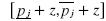, and there is a hole in the distribution of firm i of size at least as big as the hole of firm j. However, the size of the hole in firm i is bigger than the hole of firm j as firm i would not choose prices below and close to , given that they can increase the price all the way to and loose few consumer. Again, this hole in the distribution of firm i would result in an even bigger hole than the one we originally assumed was part of the best response.

Size of the support cannot be greater than 2z

Now I show that the support of the distribution cannot be smaller than 2z.

Any price p of any firm has to be "matched" by p + z or p – z in the distribution of the other firm. If the distribution were smaller than 2z, then we would have that there is a price p, in the middle of the distribution, that is not corresponded by p + z or p – z in the distribution of the other firm. By not being matched by p + z or p – z, price p cannot be in the distribution of prices and this means that there is a hole in the middle of the distribution. But as we have seen above, there cannot be holes in the distribution of any firm and therefore it is not possible that the distribution may be smaller than 2z.

Appendix C

Proof that deviations from the distribution of prices are suboptimal

Higher prices deviations

I first analyze the options of a firm, let's say firm i, to charge a price higher than the support I solved above.

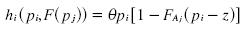
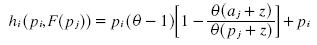
If a firm charges p_i > b_i its profits are given by the following equation:

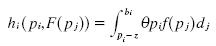
The solution to this integral is given by:

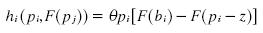
because F(p_j)=1 and p_i– z is in region A_j we can write π_i as:

but we know that 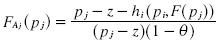where h_i = θ(a_j + z). By substituting F_Aj(p_j) we get:

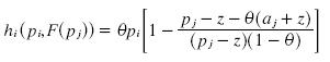
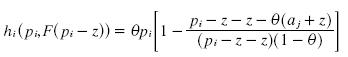
but we know fhat p_j = p_i – z, so we can substitute it and get:

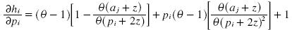
we can take the derivative of π_i with respect to p_i. If the derivative is always positive, then profits increase with the price and the firm wants to increase its price, taking us far from the prices in the distribution. If the derivative is always negative, then the firm wants to decrease its price until the distribution of the prices for the mixed strategies.

We can simplify some terms and get:

we adding terms the equation simplifies to:

this equation is negative, and therefore the profits for the firm decrease as it increases its price beyond the distribution we got above. Now we analyze a decrease in the price below the distribution of prices we got above.

Lower prices deviations

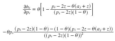
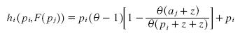
If a firm charges p_i < a_i its profits are given by the following equation:

The solution to this integral is given by:

because F ( b_j ) = 1,F (a_j ) = 0 and p_i + z is in region B_j we can write π_i as:

we know that 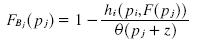where h_i = θ (a_i+ z). By substituting F_Bj (p_j) we get:

we also know that p_j = p_i + z, so we can substitute and get:

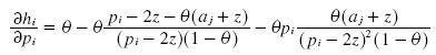
we can take the derivative of π_i with respect to p_i. If the derivative is always positive, then profits increase with the price and the firm wants to increase its price, taking us to the distribution. If the derivative is negative, then the firm wants to decrease its price below the distribution of the prices.

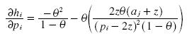
by simplifying terms, we get:

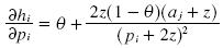
this equation is always positive, and therefore the profits for the firm increases as it increases its price towards the distribution of prices.

Appendix D (figures)

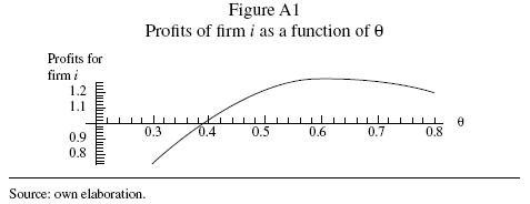
In figure A1, we can appreciate the profits for firm i in function of θ (the share of the market for firm i).

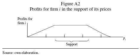
In the next figure we can appreciate the profits for firm i in function of its price.

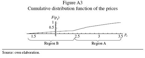
In figure A3,1 show the cumulative distribution function for both regions.