


 nueva página del texto (beta)
 Inglés (pdf)
 Artículo en XML
 Referencias del artículo
 Enviar artículo por email
 Citado por SciELO
  Similares en
SciELO
Similares en
SciELO 
 Permalink
Introduction
A project is the result of a temporary effort to create a unique product, which has an objective specified by definition of its scope; for its execution, the work is organized through a set of specific tasks, which are performed within the constraints imposed by available time, human, material and financial resources (PMI, 2013). To ensure the successful execution of complex projects, such as those of construction, they must be managed effectively.
The early history of project management occurs in the late nineteenth century when the American engineer Frederick Taylor, -who is considered as the father of scientific administration- used the tools of his profession to perform a study for the duration time of work and its remuneration. An important and innovative result of his research was to demonstrate that the performance was not improved by investing more effort and/or working hours, as it was thought at the time, but by making work more efficient by analyzing and improving basic tasks (Shultz & Schultz, 1986).
At the beginning of the twentieth century and almost simultaneously, two engineers Karol Adamiecki from Poland and Henry Gantt from United States developed graphic ways to represent the complex interdependencies of production processes: Karol invented the harmonogram and Henry Gantt the Gantt chart (Marsh, 1975; Gantt,1913); the latter first showed its effectiveness in the construction of Hoover Dam (United States) which was completed in less time than planned, and later it would become the most popular chart for representing the results of planning time (Schweckendiek et al., 2015).
Important innovations in project management were developed early in the second half of twentieth century. The American Association of Cost Engineers (AACE) was established in 1956 with the aim of improving and standardizing cost engineering best practices (Clark & Lonrezoni, 1996); AACE currently offers six certification programs and publishes the journal Cost Engineering.
A year later, firms Remington Rand and Dupont developed the Critical Path Method (CPM), represented by a complex algorithm based on graphs which allowed for the first time, to identify which processes directly determine the duration time of project. Almost simultaneously, the Office of Special Projects of the Navy of the United States of America developed the Program Evaluation Review Technique (PERT), whose innovation was the treatment of the durations of the project tasks as random variables; this same organization developed simultaneously with the PERT method, the work breakdown structure (WBS) consisting of a hierarchical tree structure that represents the division of the project work for its execution (Piquera, 2013).
The International Project Management Association (IPMA) is founded in 1965 in Switzerland, this organization was the first company specializing in project management. Four years later in the United States is founded the Project Management Institute (PMI), in order to bring together professionals in the project management field. As a result of work performed in the PMI, the Project Management Body of Knowledge (PMBOK) is published twenty years later as a set of standard terminology and project management guidelines for documenting best practices for project management; currently the PMBOK is published in eleven languages, and is widely accepted as the international standard for project management (Santiago et al., 2013).
In 1966 the Secretary of Defense of the United States of America introduced the project management Earned Value Management (EVM) method, which allows to control the execution of a project through its budget and its schedule (Humphreys, 2012). This technique consists of comparing the budgeted cost of work performed (Earned Value), with the actual cost of work performed (Actual Cost) and with the cost of work planned at the date on which the assessment is performed (Planned Value).
This allows to know how much work has been performed and how much project work needs to be finished for project completion; by means of an extrapolation of previous data an Estimate to Complete can be appraised. In the PMBOK this method has been carried out as a standard and a complete chapter is devoted to monitoring and control processes through the EVM (PMI, 2013). In Figure 1 curves representing the values used in the EVM method are showed: Planned Value (solid line), Actual Cost (dotted line) and progress made according to planned costs or Earned Value (dashed line).
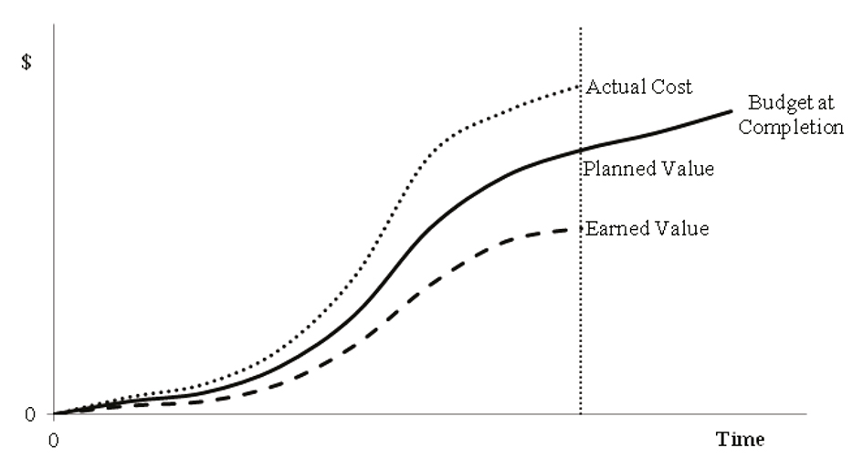
Figure 1 Curves used with earned value management method: planned value, actual cost and earned value
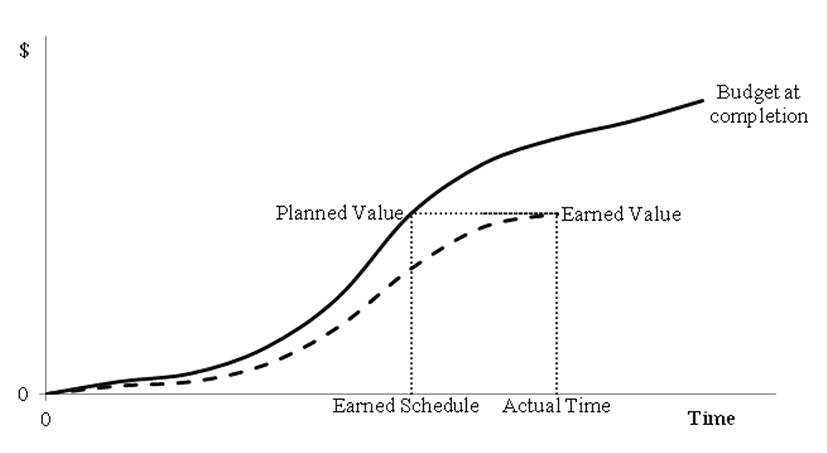
After several decades using the EVM method, project managers recognized that indicators of EVM proved to be unhelpful to control time mainly in the last third of the project duration, because the Planned Value is limited to the value of Budget at Completion. At the beginning of the twentieth-first century, an extension of the EVM method to perform an assessment on project time performance was developed by the American physicist Walt Lipke; today this extension is known as the Earned Schedule (ES) method. In this method, instead of comparing costs, time periods are compared: the actual number of time periods that have been elapsed (Current Time) with the number of time periods related to the budgeted cost of work that have been performed (Earned Schedule) (Lipke, 2003). In Figure 2 the curves representing the values used in (ES) method are presented as: Planned Value (solid line) and Earned Value according to the planned cost (dashed line).
The importance of project management in construction is that this is a nomadic industry, where operating conditions are generally being barely implemented, and it is very difficult to reach the optimization phase; besides the production cycle is not repeated and is generally very long. These conditions make the construction activity tend to be more susceptible to have more sources of uncertainty than those other industries which operate as a regular basis in factories and implement continuous, uniform and more predictable operation cycles (Sears et al., 2008). All this makes controlling construction projects, gain particular relevance during the building phase.
Traditionally the backbone of control during the building phase of projects has focused on monitoring the project duration and the costs incurred, because they represent important performance parameters for both the customer and the firm responsible of managing the project. Breach on project delivery time is usually one of the main causes of lawsuits against construction firms (Solís et al., 2015); and achieving expected profits, is but few exceptions, the main goal of builders.
It is a common practice in construction firms, a periodic assessment of progress for the work performed, as well as costs incurred; however, small and micro construction firms, which do not have an organizational structure of enough size, specialty and maturity, usually do not often take advantage of data collected periodically, through analysis, forecasting and implementing actions tending to make the necessary corrections to conclude all work on time and without decreasing profit (Al-Momani, 2000).
The aim of this study was to evaluate the effectiveness of project management methods: Earned Schedule and Earned Value; which are used to control time and cost, respectively, in construction projects in southeastern Mexico.
Methodology
The analysis unit was the construction project managed in the Yucatan Peninsula, Mexico by kind of firm classified by size as micro or small. The sample consisted of six projects, which were carried out by five construction firms. Table 1 presents for each project: the planned duration time, the direct cost originally estimated, its description, the firm that built and the firm size; it is important to observe that all the costs mentioned in this work are presented in US dollars. The classification for the firm size was defined according to the criteria of the National Institute of Statistics and Geography of Mexico (INEGI, 2009). The selected firms were those which were interested in participating in the research, and had at least one construction project during research period; the requirements of the projects were to have a minimum duration of three months and a minimum estimated direct cost of $55,000.

The first part of the methodology was to conduct an assessment of the control processes of time and cost, that participating firms routinely perform during construction of their projects. For the first part, a survey was carried out to the responsible for these processes by using a questionnaire of 32 items; 16 items for responsible of the time control, and 16 items to the responsible of cost control; the used instrument was designed following the guidelines of the PMBOK Guide (PMI, 2013); specifically, on sections: 6.6 Develop schedule and 7.4 control costs. The scale used was nominal and classified into three categories of practices: those that can be considered good, those which can be considered acceptable and those that can be considered deficient; values of 3, 2 and 1, were assigned to these categories respectively; it is important observing that when a firm said to carry out more than one action in the same process, the assigned value was limited to a maximum of 3 (corresponding to good practice). In order to compare firms, a global assessment was obtained for each one, it was calculated as the total sum of values for both control processes of time and cost control; without using any weighting that would differentiate the questions. The variation coefficient was calculated with these values.
In the second part of methodology, the performance indicators were measured and predictors were calculated during the construction phase of sampled projects. All six projects were divided randomly into two groups: the first one provided with the predictors of time and cost during construction phase (it can be considered that this group was manipulated experimentally); and the second one was not provided with such predictors, so processes for control time and cost were performed in the usual way. The first group consisted of projects B, C and D, and the second group consisted of projects A, E and F. The predictors were provided to firms classified in the first group, at the time when the original scheduled progress were of: 20%, 40 %, 60 % and 80%. In Table 1 Italic format has been used in the three lines corresponding to the projects that were given their predictors, action that will be hereinafter referred as the feedback.
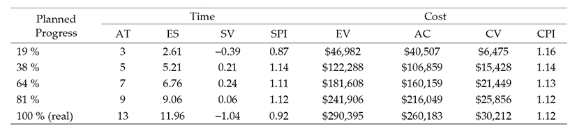
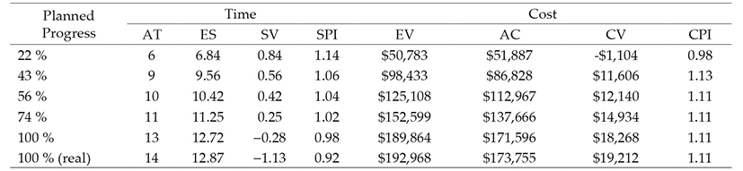
The Earned Schedule method was used for measuring projects performance from the point of view of its duration (Lipke, 2003). Earned Schedule Indicators: Schedule Variance (SV) and Schedule Performance Index (SPI) were calculated every week using equations 1 and 2:
Where AT is the Actual Time and ES is the Earned Schedule which is obtained with equation 3
Where C is the number of complete time periods and I is time period fraction, which is calculated with equation
Where BCWP is the Budgeted Cost of Work Performed and BCWS is the Budgeted Cost of Work Scheduled. From these indicators the predictor of time Independent Estimate at Completion (IEAC) was obtained every week with equation 5
Where Planned Duration is denoted with PD. In the same way, measuring performance of projects, from the point of view of its cost, was carried out with the Earned Value method (PMI, 2013).
Earned Value Indicators were calculated every week: Cost Variance (CV) and Cost Performance Index (CPI), with equations 6 and 7
Where EV is the Earned Value and AC represents Actual Cost. Cost Estimate at Completion (EAC) predictor were calculated from these indicators each week, with equation 8
Where ETC is the Estimate to Complete, which was calculated with equation 9
Where Budget at Completion is denoted by BAC.
According to performance indicators discussed above, the interpretation of its values is presented in Table 2. The table space has been divided into an area of good performance (unshaded), and areas where the performance shows delays, cost overruns or both (shaded gray).

The relationship between the predicted values and planned time and cost for each project were calculated weekly. These values were charted for a better understanding of the performance of project execution. Values with ratio less or equal to 1 mean that the project had a good performance.
Student's t-test was used to analyze if the mean values for performance indicators (SPI and CPI) were significantly different between the group of projects that received a feedback and those that not received it. The tests were applied assuming equal variances in the two groups and test were repeated assuming unequal variances. An acceptable significance level of 1 % was considered because data were too few.
Results
Tables 3 and 4 present a summary of results for the assessment of time and cost control processes that participating firms performed on a regular basis during the execution of their projects. For comparison purpose, the last rows of these tables contain the overall assessment of each construction firm.


The performance indicators of project management of time and costs were calculated weekly from data collected in site and from accounting departments of firms, respectively. For projects managed by firms that received feedback, these indicators are presented in Tables 5, 6 and 7; because of space economy, only data for weeks in which feedback was given to firms (approximately for planned progress of 20, 40, 60 and 80%) are included in such tables; the indicators for the week in which project completion (100%) was planned and for those which actually concluded (100 % real) are also included. In Tables 5, 6, 7, 8, 9 and 10, costs are in US dollars and weeks in which projects fall out of area of good performance are shaded, according to the criteria presented in Table 2.
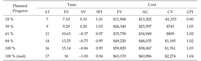


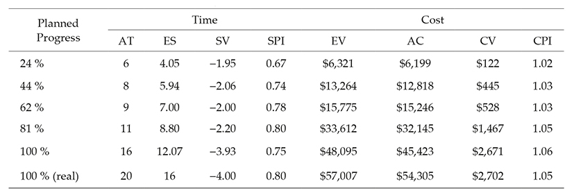
Likewise, in Tables 8, 9 and 10 performance indicators calculated for projects implemented by firms that have received no feedback.
Weekly predictors for time to completion and total cost of each project were calculated from the performance indicators. For projects managed by firms receiving feedback, the following curves are shown in Figure 3: relationship between the predicted time to completion and the time originally planned (solid line); the relationship between the predicted total cost and cost originally estimated (with dashed line); additionally, week corresponding to the Planned Duration of the project is marked with a straight vertical line. As discussed in the methodology section, when plotted values are less or equal than 1 (predicted value less or equal than the planned value), it means that the project is in the area of good performance.

Figure 3 Relationship between time and cost values predicted and planned for projects with feedback (B, C and D)
Similarly, for projects managed by firms that received not feedback, the curves representing the relationship between predicted time to completion and originally planned time; and the relationship between the total cost and originally estimated predicted cost are presented in Figure 4.

Figure 4 Relationship between time and cost values predicted and planned for projects without feedback (A, E, and F)
Table 11 shows a summary of performance results observed in the six projects. The last two columns correspond to the performance indicators calculated in the weeks when projects concluded; gray shading means that the project was outside the area of good performance and italic font type means that the project received a feedback.

Table 12 shows results of t-Student for testing equality of means on final indicators SPI and CPI (see Table 11); the grouping factor analyzed was the fact of receiving feedback on the predictors. We can see a significant difference (α≤ 0.01) for the SPI indicator (time) and not that significant for CPI (cost) for both equal and not equal variances.

Discussion
According to surveyed data on time control, firm 5 (managing project F) which stated having the best practices, that can be summarized as follows: measures weekly performed work, compared against planned work, forecasts time to completion date and if necessary takes exceptional measures, such as increasing the number of workers or make more emphasis on work supervision. In the case where project is delayed, the firm did not mention if it identifies the critical activities that were causing delays, nor if it makes a rescheduling for the missing work to be performed. In order of best to worst the other four firms occupied the following positions: 1 (implementing project A), 4 (Project E), 2 (projects B and C) and 3 (Project D); see global assessment in Table 3. According to diagnosis on cost control, also the firm 5 stated to have the best practices, which can be summarized as follows: calculates the weekly cost incurred, compared to the planned cost, generates cost accounts by resource type, and when the project has overruns it reviews the actual cost of resources. This firm did not state that the forecast made for final cost estimate of the project and its labor productivity were reviewed; however, the importance of measuring productivity, as a means of monitoring compliance with the goals has been highlighted in several previous studies (Takim et al., 2003; Chan & Chan, 2012). Again, in order of best to worst the other four firms occupied the following positions: 3, 1 and 4 in the same position and 2; see global assessment on Table 4.
In Figure 5 is presented the global assessment of the time and cost control processes for the five firms. It can be observed that assessing time control processes had greater variability than in the cost; in the first case was obtained a variation coefficient of 0.23 and 0.10 in the second.

The six projects were completed in more time than originally scheduled. However, those who received feedback performed better, it can be noted in two ways: in most of weeks, these projects were in the area of good performance (SPI ≥ 1); and the final values of SPI projects receiving feedback were significantly higher compared to those in the other group (Table 12).
Figure 6 depicts the possible effects on time performance indicator (SPI) having received feedback and magnitude of project cost. It can be observed, as has been written above, that the project group with feedback (marker on black color) has performed better than the group that did not have it (white label). For each group, it can also be observed that lower cost projects were performed better; and that the combination of high cost and not having feedback resulted in projects having the worst performance of the study (project A SPI equal to 0.73 and 40 days of delay). The size of the work in terms of cost and/or extension has an influence in construction performance on firms; this has been previously reported by Botero and Alvarez (2004) in housing projects.

Similarly, in Figure 7 is showed the possible effects of having feedback and the global assessment of time control on performance indicator (SPI). It is expected that projects implemented by the firms with the highest global assessment (F, A and E) had higher SPI; however, in this figure, such effect is not observed, so the interpretation could be that the feedback effect was much greater than making use of good practices for control time stated by the firms. In a previous study in the same region, was found moderate correlation between the application of good management practices and performance in project implementation; a correlation coefficient of 0.60 was reported between good practices in monitoring and enforcement planned duration of project (Solís et al., 2015).

Comparing Figures 3 and 4, clearly can be observed that the projects having feedback (Figure 3) had a closer to 1.0 relationship between project duration predicted and planned, rather than those without feedback (Figure 4); this means that those had feedback, generally were in or nearby the good performance area.
Moreover, the six projects had a final direct cost less than originally estimated (Table 11). In most of weeks, all projects were in the good performance area (CPI ≥ 1); and the final CPI values for projects in the group which received feedback were not significantly different (α≤ 0.01) to those belonging to the other group (Table 12).
The above results suggest an independence between indicators of time and cost performance, such thing in the context of this study could have the following explanations:
No information on indirect costs was obtained, regularly indirect costs are more affected by delays because they tend to increase along with a greater project duration.
All firms paid labor per unit prices or piecework, which makes labor cost be independent of productivity and duration.
Because of firms size (micro and small) is common that the owners of firms be responsible of cost incurred control as a way to ensure its profits.
The firms have practice on overestimating costs at the planning stage, as a way to hide the client a fraction of their profits.
This last point has been reported as a common practice in the context where the study was performed (Morfin, 2015); internationally it has been reported that construction firms tend to overestimate the direct costs as a risk management strategy generated by uncertainty especially in the labor costs (Shiner, 2013).
Conclusions
For those projects where Earned Schedule method was applied -including calculation of indicators and feedback on predictors to responsible of each firm- the performance relative to total duration was significantly better than those projects managed in the usual way, without using the ES.
In projects where Earned Value Management method was applied, -including calculation of indicators and feedback on predictors to responsible of each firm- no significant improvement in performance relative to direct cost was observed regarding projects that where managed in the usual way.
In the context of this study -micro and small firms, payment of labor per unit prices and not considering indirect costs- an independence between performance indicators of time and cost was found.
Therefore the study results showed that constructions firms need to emphasize management for project execution time, by using modern engineering methods. On the other hand, constructions firms’ primary goal is obtaining a desirable profit, so the cost management results showed to be adequate by using traditional means.

