Research
Other Areas in Physics
The investigation of a classical particle in the presence of
fractional calculus
Won Sang Chunga
S. Zareb
H. Hassanabadib
c
J. Křížc
E. Maghsoodid
aDepartment of Physics and Research Institute of
Natural Science, College of Natural Science, Gyeongsang National University,
Jinju 660-701, Korea.
bFaculty of Physics, Shahrood University of
Technology, Shahrood, Iran.
c Department of Physics, University of Hradec
Králové, Rokitanského 62, 500 03 Hradec Králové, Czechi
d Department of Physics, Faculty of Science,
Lorestan University, Khoramabad, Iran. e-mail:
h.hasanabadi@shahroodut.ac.ir
Abstract
In this article, by applying a preliminary and comprehensive definition of the
fractional calculus, its effect on different aspects of physics is specified, as
in the case of Laplace transforms, Riemann-Liouville, and Caputo derivatives.
Applications of the fractional calculus in studying the dynamics of particle
motion in classical mechanics are investigated analytically. Furthermore, we
compare our results with those obtained from the usual methods and we show that
both solutions coincide provided the fractional effects are removed.
Keywords: Fractional calculus; fractional classical mechanics; Riemann-Louville fractional derivative
PACS: 45.50.Dd; 45.05.+x; 45.20.Jj
1.Introduction
The calculus of differentiation and integration is known as the fractional calculus.
The fractional derivatives for the first time were proposed by Gottfried Wilhelm
Leibniz in (1695) 1. Now the
fractional calculus has been considered as a new tool for modeling the complex
systems 2-16. Since then, the fractional
derivative was examined for various functions. The fractional derivative of the
exponential function and the power function, respectively, are obtained by Liouville
in (1832) and Riemann in (1847) 1.
Many researchers consider an integral form for the fractional derivative and the two
most popular types of fractional derivatives are Riemann-Louville and Caputo. The
fractional derivative has many interesting and unexpected properties; for example,
under special conditions, the derivative of a constant can be nonzero, such as the
case of the Riemann-Liouville fractional derivative. On the other hand, the Caputo
derivative of a constant, as the ordinary derivative, vanishes. For further
information on fractional calculus, the interested reader is referred to Refs. 17-21.
Different definitions of fractional derivatives can be proposed, each with remarkable
properties 22-26, all of them valid and
mathematically acceptable.
In Ref. 37, the authors proposed a
new fractional differential equation to describe the mechanical oscillations of a
simple system and they analyzed the systems mass-spring and spring-damper. In Ref.
38, the authors proposed a
fractional differential equation to describe the vertical motion of a body through
the air. Two-dimensional projectile motion in a free and in a resistive medium were
investigated using the so-called conformable derivative in Ref. 39. The motion of
a projectile by using the Riemann-Liouville fractional derivative and the Caputo
approach is studied in Refs. 40,41.
Recently, using fractional calculus, the dynamics of a particle have been studied for
resisted horizontal motion within a viscoelastic medium and in the presence of a
uniform force 22. Moreover, in
Ref. 23, in the framework of
conformable fractional quantum mechanics, the three-dimensional fractional harmonic
oscillator is studied and by using an effective and efficient formalism, Schrödinger
equation, probability density, probability flux and continuity equation have been
investigated and in Ref. 24.
Fractional calculus has also been studied for the Dirac equation, the resulting wave
function, and the energy eigenvalue equation.
There are different methods to solve fractional differential equations analytically.
One of the most common, simple, and practical methods used is the Laplace transform
25. In this paper, the Laplace
transform of fractional operators is represented, and some related formula is
introduced. Fractional calculus has been considered for modeling viscoelastic
systems that cover various fields and subjects 22. Here, we show that the proposed fractional model has
a better result as compared to that of the non-fractional models have shown for
probing the different aspects of mechanical physics.
This work is organized as follows. We first review the fractional calculus in Sec. 2.
Next, we investigate dynamics of a particle within a viscoelastic medium in Sec. 3.
In Sec. 4, by considering a retarding force proportional to the fractional velocity,
vertical motion of a body in a resisting medium is studied and in the last section,
to provide a better understanding of the motion of a projectile in a resisting
viscoelastic medium, we will discuss it under the condition that there exists a
retarding force proportional to the fractional velocity.
2.Introduction to Fractional Calculus
The Riemann-Louville fractional integral is defined as
I0 |xαfx=1Γα∫0xx-ξα-1fξdξ x>0,
(1)
where 0<α<1 and f(x) is a continuous function.
Also the Caputo fractional derivative is introduced as 22
D0 |tαft=1Γn-α∫0tt-ξn-ν-1dndξnfξdξ,
(2)
where n=[ν]+1 and [x] implies a Gauss symbol.
The Laplace transform of Caputo fractional derivative can be represented by the
following form
LDtαxt=smFs-sm-1x0-sm-2x'0-…-xm-10sm-α,
(3)
and by inserting α = 1 and m = 2 in Eq (1), we have
LDt2xt=s2Fs-s x0-x'0.
(4)
The Mittag-Leffler functions and the generalized Mittag- Leffler functions for α´,β´
> 0 and z∈C are defined as 34
Eα'z=∑n=0∞znΓnα'+1,
(5)
Eα',β'z=∑n=0∞znΓnα'+β'.
(6)
For α',β'>0, a∈R and sα'>a inverse Laplace transform formula has the form
L-1sα'-β'sα'+a=tβ'-1Eα',β'-atα'.
(7)
3.Resisted motion of a particle in a viscoelastic medium
Now let us investigate the dynamics of a particle in a viscoelastic medium. In
reality, per cycle of motion the part of the energy is destroyed. In the other
words, the measure of damping is determined by the amount of energy lost.
Experimentally, we can consider the horizontal motion in a viscoelastic medium as the
simplest example of the resisted motion of a particle. By considering a general
order of viscoelastic damping, the frictional force takes the following form
Fα=-CDtαxt, 0≤α<1.
(8)
In order to be consistent with the time dimensionality, we consider, the fractional
derivative operator as
ddt→1C11-αdαdtα,
(9)
where C1 represents the fractional time in the system 37. Then, in Eq. (8), we change
C to (C/C11-α).
In this case, the Newtonian equation satisfies the equation of motion as follows
mDt2xt=-CC11-αDtαxt,
(10)
with the following initial conditions
x'0=V0, x0=0.
(11)
On the other hand we know that Fs=Lxt, therefore we have
LmDt2xt=-LCC11-αDtαxt,
(12)
then by substituting Eq. (1) and Eq. (2) into Eq. (12), we find the following
relation:
ms2Fs-sx0-x´(0)=-CC11-αsαFs-sα-1x(0)
(13)
which, upon substitution of Eq. (11), becomes
ms2Fs-V0=-CC11-αsαFs,
(14)
where
Fs=mV0ms2+CC11-αsα.
(15)
Therefore, we can write
xt=L-1Fs=V0L-11s2+CmC11-αsα,
(16)
which can be compared with Eq. (5) to obtain the following parameters:
α'=2-α, β'=2, a=CmC11-α,
(17)
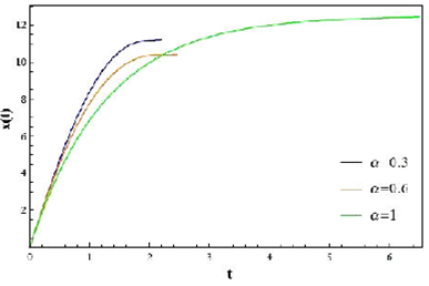
after which the solution for x(t) reads
xt=V0tE2-α-CmC11-αt2-α=V0t1Γ(2)+-CmC11-αt2-αΓ(4-α)+-CmC11-αt2-α2Γ(6-2α)+-CmC11-α22-α3Γ(8-3α)+…
(18)
In Fig. 1, x (t) with three different values of
α as a function of t with parameters C = 0.8, C1 = 1.2, m = 1 and
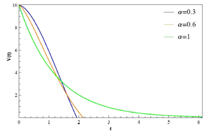
V0 = 10 has been plotted. Using the equation above, the velocity can
be written as
Vt=1mt-αV0mtαE2-α,2-CmC11-αt2-α-CC11-αt2E2-α,3-α-CmC11-αt2-α-E2-α,4-α-CmC11-αt2-α
(19)
In Fig. 2, we have plotted V(t) with three
different values of α as a function of t with parameters C = 0.9, C1 =
1.2, m = 1 and V0 = 10. Then, we have obtained the acceleration as
at=1m2CC11-αt1-2αV0CC11-αt2E2-α,4-2α-CmC11-αt2-α+(3+α)CC11-αt2E2-α,5-2α×-CmC11-αt2-α-CC11-αt2E2-α,6-2α-Cmc11-α+mtαE2-α,3-α-CmC11-α-E2-α,4-α-CmC11-αt2-α
(20)
Special cases:1) For α=1/2
Recalling Eqs. (4) and (17) and substituting into Eq. (18), the obtained solution
becomes
xt=V0 t E32, 2-CmC112t32=V0t1Γ2+-CmC112t32Γ72+-CmC112t322Γ5+-CmC112t323Γ132+....
(21)
So, velocity and acceleration can be calculated as follows:
Vt=1mV0mE32,2-CmC112t32+CC112t32E32,52-CmC112t32+E32,72-CmC112t32
(22)
at=12m2CC112tV0-5mE32,52-CmC112t32+2CC112t32E32,3-CmC112t32+5mE32,72-CmC112t32-5CC112t32E32,4-CmC112t32+5CC112t32E32,5-CmC12t32
(23)
in view of other special approaches as follows 2) For C = 0, Eq. (21) leads
xt=V0 t
(24)
4.Vertical motion of a body in a resisting medium
Now let us consider the vertical motion of a body in a resisting medium in which
there exists a retarding force proportional to the fractional velocity. In this
case, we consider that the body is projected downward with zero initial velocity
v(0) = 0 in a uniform gravitational field. Then the equation of motion is given
by
mDt2yt=mg-CC11-αDtαyt, 0<α≤1
(25)
with the following initial condition
y0=y0, y'0=0
(26)
Taking the Laplace transform of both side of the Eq. (25), we get
ms2Fs-sy0-y´(0)=mgs-CC11-α×sFs-y0s1-α.
(27)
Solving the Eq. (27) with respect to f (s), we have
Fs=gs3+CmC11-αsα+1+y0s+CmC11-αsα-1+CmC11-αy0s3-α+CmC11-αs,
(28)
which can be rewritten as
gs3+CmC11-αsα+1β´=3, α´=2-α,y0s+CmC11-αsα-1β´=1, α´=2-α,Cy0mC11-αs3-α+CmC11-αsβ´=3- α´=2-α
(29)
Using the inverse Laplace transform yt=L-1F(s), we have
yt=y0E2-α,1-CmC11-αt2-α+gt2E2-α,3-CmC11-αt2-α+CmC11-αy0t2-α×E2-α,3-α-CmC11-αt2-α
(30)
For the special case when α = 1, we obtain
yt=y0E1,1-Cmt+gt2E1,3-Cmt+Cmy0t2-αE1,2-Cmt
(31)
which can be expanded in series as
yt=y0+12!gt2+13!-Cmgt3+14!Cm2gt4+...,
(32)
so that in the limit of C → 0,
yt=y0+12!gt2.
(33)
On the other hand, for α = 1/2 we will have
yt=y0E32,,1-CmC112t32+gt2E32,3-CmC112t32+CmC112y0t32E32,52-CmC112t32.
(34)
For simplicity above equation can be written as
yt=y01Γ(1)+gt21Γ(2)+-CmC112t32Γ92+C2m2C1t3Γ(6)+…
(35)
where, after using Γ(3)=2!, the result is read as
yt=y0+12gt2-CmC112gt72Γ92+…
(36)
5.Motion of a projectile in a resisting medium
In this section we are interested in considering motion of a projectile in a
resisting viscoelastic medium in which there exists a retarding force proportional
to the fractional velocity. In this case we have the following equations
mDt2x(t)=-CC11-αDtαx(t),mDt2y(t)=-mg-CC11-αDtαy(t),0<α<1
(37)
with the initial conditions
x(0)=0,y(0)=0,x'(0)=V0cosθ,y'(0)=V0sinθ.
(38)
Taking the Laplace transform of both on both sides of Eq. (39), we can find
Fs=V0cosθms2+CC11-αsα,
(39)
Gs=-mgms3+CC11-αsα+1+V0sinθms2+CC11-αsα.
(40)
where F(s) and G(s) are Laplace transforms of x(t) and y(t) respectively. Using the
inverse Laplace transform and properties of Mittag-Leffler function, we have
xt=V0cosθtE2-α,2-CmC11-αt2-α,
(41)
yt=-gt2E2-α,3-CmC11-αt2-α+V0sinθtE2-α,2-CmC11-αt2-α
(42)
In Fig. 3, we have plotted x(t) with three
different values of α as a function of t with parameters C = 0.8,
C1 = 1.2, m = 1, θ=π/6 and V0 = 10. Also, in Fig.
4, we have plotted 𝑦(t) with three different values of
α as a function of t with parameters C = 0.8, C1 = 1.2, m = 1, g=10, θ=π/6 and V0 = 10.
Differentiating x(t) and y(t) with respect to the time, the velocity can be
calculated as
x´t=1mt-αV0cosθmtαE2-α,2-CmC11-αt2-α-CC11-αt2E2-α,3-α-CmC11-αt2-α-E2-α,4-α-CmC11-αt2-α
(43)
and
y´t=1mt-α-2gmt1+αE2-α,3-CmC11-αt2-α-2CC11-αgt3E2-α,5-α-CmC11-αt2-α+mtαV0sinθE2-α,2-CmC11-αt2-α-CC11-αt2V0sinθE2-α,3-α-CmC11-αt2-α+CC11-at2gt+V0sinθE2-α,4-α-CmC11-α
(44)
If we denote the range and the time required for the entire trajectory by R´ and T´
respectively, the following representation is obtained
yt=T'=0.
(45)
Now consider the case that α = 1- ε and ε is sufficiently small. In this case we
have
E2-α,l~1-CmC1εl-1e-CmC1εt-∑n=0l-2-CmC1εtn+ε∑n=0∞nΓn+lFn+l-1-CmC1εn+ε Int∑n=0∞nΓ(n+l)-CmC1εtn
(46)
By using Eqs. (45) and (46), up to a first order in ε, we have
T'=2V0sinθg1-CV0sinθ3mgC1ε+ε2CV02sin2θ3mg2C1ε-γ+136+ln2V0sinθg,
(47)
which, when α goes to 1, can be simplified into
T'→T=2V0sinθg1-CV0sinθ3mgC1ε.
(48)
The range is obtained from the relation R´= x(T´) as
R'=V02sin2θg1-4CV0sinθ3mgC1ε+ε2CV03sin2θcosθ9mg2C1ε,
(49)
2 which can be reduced, when α goes to 1, to we can also have
R'→R=V02sin2θg1-4CV0sinθ3mgC1ε.
(50)
Therefore, the change due to the fractional resistance is given by
ΔR=R'-R=ε2CV03sin2θcosθ9mg2C1ε>0.
(51)
Thus, the range becomes larger for the fractional resistance when compared with the
linear resistance case.
6.Conclusion
In this article, we have considered fractional calculus as a new tool in studying
interesting aspects of classical mechanics. First, we have briefly discussed the
basic concepts of fractional calculus and we have presented an interpretation of
fractional derivative and solution of fractional equations analytically. Then, by
considering the modeling of viscoelastic systems within the fractional calculus
framework, we have investigated applications of this approach in three different
problems in classical mechanics including the study of resisted motion of a particle
in a viscoelastic medium, the vertical motion of a body in a resisting medium and
the motion of a projectile in a resisting medium. The obtained results satisfy the
ordinary results of classical mechanics in. It has also been proved that the
ordinary solutions are obtained provided the fractional effects are removed. Thus,
the results demonstrate that the proposed fractional model presents an enhanced
description as compared to that of the non-fractional models have shown when probing
the different aspects of mechanical physics.
Acknowledgement
The authors thank the referee for a thorough reading of our manuscript and for
constructive suggestions. HH and JK are grateful for the institutional support of
the Faculty of Science, University of Hradec Králové, research team “Mathematical
physics and differential geometry”.
References
1. M. Dalir and M. Bashour, Applications of fractional calculus,
Appl. Math. Sci. 4 (2010) 1021.
[ Links ]
2. M. M. Meerschaert and C. Tadjeran, Finite difference
approximations for two-sided space-fractional partial differential equations,
Appl. Numer. Math. 56 (2006) 80.
https://doi.org/10.1016/j.apnum.2005.02.008
[ Links ]
3. H. Jafari, C.M. Khalique, and M. Nazari, An algorithm for the
numerical solution of nonlinear fractional-order Van der Pol oscillator
equation, Math. Comput. Model. 55 (2012) 1782.
https://doi.org/10.1016/j.mcm.2011.11.029.
[ Links ]
4. H. Jiang et al., Analytical solutions for the multi-term
time-space Caputo-Riesz fractional advection-diffusion equations on a finite
domain, J. Math. Anal. Appl. 389 (2012) 1117.
https://doi.org/10.1016/j.jmaa.2011.12.055.
[ Links ]
5. R. Almeida and D. Torres, Calculus of variations with fractional
derivatives and fractional integrals, Appl. Math. Lett. 22 (2009) 1816.
https://doi.org/10.1016/j.aml.2009.07.002.
[ Links ]
6. M. Gülsu, Y. Öztürk, and A. Anapali, Numerical approach for
solving fractional relaxation-oscillation equation, Appl. Math. Model. 37 (2013)
5927. https://doi.org/10.1016/j.apm.2012.12.015.
[ Links ]
7. D. Baleanu, Fractional variational principles in action, Phys.
Scr. 136 (2009) 014006.
https://doi.org/10.1088/0031-8949/2009/T136/014006.
[ Links ]
8. A. Iomin, Fractional-time quantum dynamics, Phys. Rev. E 80
(2009) 022103. https://doi.org/10.1103/PhysRevE.80.022103.
[ Links ]
9. W. Bu, Y. Tang and J. Yang, Galerkin finite element method for
two dimensional Riesz space fractional diffusion equations, J. Comput. Phys. 276
(2014) 26. https://doi.org/10.1016/j.jcp.2014.07.023.
[ Links ]
10. W. Bu et al., Finite difference/finite element method for
twodimensional space and time fractional Bloch-Torrey equations, J. Comput.
Phys. 293 (2015) 264.
https://doi.org/10.1016/j.jcp.2014.06.031.
[ Links ]
11. M. Efe, Battery power loss compensated fractional order sliding
mode control of a quadrotor UAV, Asian J. Control 14 (2012) 413.
https://doi.org/10.1002/asjc.340.
[ Links ]
12. Y. Li, Y. Chen and H. Ahn, Fractional-order iterative learning
control for fractional-order linear systems, Asian. J. Control 13 (2011) 54.
https://doi.org/10.1002/asjc.253.
[ Links ]
13. B. Jin et al., The Galerkin finite element method for a
multiterm time-fractional diffusion equation, J. Comput. Phys. 281 (2015) 825.
https://doi.org/10.1016/j.jcp.2014.10.051.
[ Links ]
14. F. Mainardi and G. Spada, Creep, relaxation and viscosity
properties for basic fractional models in rheology, Eur. Phys. J. Spec. Top. 193
(2011) 133. https://doi.org/10.1140/epjst/e2011-01387-1.
[ Links ]
15. R. Lewandowski and B. Chorażyczewski, Identification of the
parameters of the Kelvin-Voigt and the Maxwell fractional models, used to
modeling of viscoelastic dampers, Comput. Struct. 88 (2010) 1.
https://doi.org/10.1016/j.compstruc.2009.09.001.
[ Links ]
16. R. Lewandowski and Z. Pawlak, Dynamic analysis of frames with
viscoelastic dampers modelled by rheological models with fractional derivatives,
J. Sound Vib. 330 (2011) 923.
https://doi.org/10.1016/j.jsv.2010.09.017.
[ Links ]
17. A. Kilbas, H. Strivatava and J. Trujillo, Theory and Application
of Fractional Differential Equations 1st ed. (Elsevier Science, Amsterdam,
2006).
[ Links ]
18. I. Pdolubny, Fractional Differential Equations 1st ed. (Academic
Press, New York, 1998).
[ Links ]
19. R. Hilfer, Application of fractional Calculus in Physics (World
Scientific, Singapore, 2011), https://doi.org/10.1142/3779.
[ Links ]
20. R. Herrmann, Fractional calculus, 1st ed. (World Scientific,
Singapore, 2011), https://doi.org/10.1142/8072.
[ Links ]
21. K. Diethelm, The Analysis of Fractional Differential Equations
(Springer-Verlag, Berlin, 2010),
https://doi.org/10.1007/978-3-642-14574-2.
[ Links ]
22. W. S. Chung and H. Hassanabadi, Dynamics of a Particle in a
Viscoelastic Medium with Conformable Derivative, Int. J. Theor. Phys. 56 (2017)
851. https://doi.org/10.1007/s10773-016-3228-z.
[ Links ]
23. F. S. Mozaffari, H. Hassanabadi, H. Sobhani and W. S. Chung, On
the Conformable Fractional Quantum Mechanics, J. Korean Phys. Soc. 72 (2018)
980. https://doi.org/10.3938/jkps.72.980.
[ Links ]
24. F. S. Mozaffari, H. Hassanabadi, H. Sobhani and W. S. Chung,
Investigation of the Dirac Equation by Using the Conformable Fractional
Derivative, J. Korean Phys. Soc. 72 (2018) 987,
https://doi.org/10.3938/jkps.72.987.
[ Links ]
25. I. Podlubny, Fractional differential equations: an introduction
to fractional derivatives, fractional differential equations, to methods of
their solution and some of their applications 198 (Academic press
1998).
[ Links ]
26. E. C. Grigoletto and E. C. de Oliveira, Fractional Versions of
the Fundamental Theorem of Calculus, Appl. Math. 4 (2013) 23.
https://doi.org/10.4236/am.2013.47A006.
[ Links ]
27. D. Baleanu and T. Avkar, Lagrangians with linear velocities
within Riemann-Liouville fractional derivatives, Nuovo Cimento B 119 (2004) 73.
https://doi.org/10.1393/ncb/i2003-10062-y.
[ Links ]
28. K. Diethelm, Efficient Solution of Multi-Term Fractional
Differential Equations Using P(EC)m E Methods, Computing 71 (2003)
305. https://doi.org/10.1007/s00607-003-0033-3.
[ Links ]
29. K. Diethelm, N.J. Ford, and A.D. Freed, Detailed Error Analysis
for a Fractional Adams Method, Numer. Algorithms 36 (2004) 31.
https://doi.org/10.1023/B:NUMA.0000027736.85078.be.
[ Links ]
30. S. Mulish and D. Baleanu, Hamiltonian formulation of systems
with linear velocities within Riemann-Liouville fractional derivatives, J. Math.
Anal. Appl. 304 (2005) 599.
https://doi.org/10.1016/j.jmaa.2004.09.043.
[ Links ]
31. F. Barpi and S. Valente, Creep and fracture in concrete: a
fractional order rate approach, Eng. Fract. Mech. 70 (2002) 611.
https://doi.org/10.1016/S0013-7944(02)00041-3.
[ Links ]
32. S. Mulish and D. Baleanu, Formulation of Hamiltonian Equations
for Fractional Variational Problems, Czechoslov. J. Phys. 55 (2005) 633.
https://doi.org/10.1007/s10582-005-0067-1.
[ Links ]
33. D. Baleanu and S. Mulish, Lagrangian Formulation of Classical
Fields within Riemann-Liouville Fractional Derivatives, Phys. Scr. 72 (2005)
119. https://doi.org/10.1238/Physica.Regular.072a00119.
[ Links ]
34. D. Craiem et al., Fractional Calculus Applied to Model Arterial
Viscoelasticity, Lat. Am. Appl. Res. 38 (2008) 141.
[ Links ]
35. R. Churchill, Operational Mathematics 3rd ed. (McGraw-Hill, New
York, 1972).
[ Links ]
36. S. Kazem, Exact Solution of Some Linear Fractional Differential
Equations by Laplace Transform, Int. J. Nonlinear Sci. 16 (2013)
3.
[ Links ]
37. J. F. Gómez-Aguilar, J. J. Rosales-García, J. J.
Bernal-Alvarado, T. Córdova-Fraga and R. Guzmán-Cabrera, Fractional mechanical
oscillators, Rev. Mex. Fis., 58 (2012) 348.
[ Links ]
38. J. J. R. García, M. G. Calderon, J. M. Ortiz and D. Baleanu,
Motion of a particle in a resisting medium using fractional calculus approach,
Proc. Romanian Acad. A, 14 (2013) 42.
[ Links ]
39. A. O. Contreras, J. J. R. García, L. M. Jiménez and J. M.
Cruz-Duarte, Analysis of projectile motion in view of conformable derivative,
Open Phys. 16 (2018) 581.
https://doi.org/10.1515/phys-2018-0076.
[ Links ]
40. B. Ahmad, H. Batarfi, J. J. Nieto, Ó. Otero-Zarraquiños and W.
Shammakh, Projectile motion via Riemann-Liouville calculus Adv. Diff. Eqs., 2015
(2015) 63. https://doi.org/10.1186/s13662-015-0400-3.
[ Links ]
41. A. Ebaid, Analysis of projectile motion in view of fractional
calculus, Appl. Math. Model. 35 (2011) 1231.
https://doi.org/10.1016/j.apm.2010.08.010.
[ Links ]


 nova página do texto(beta)
 Inglês (pdf)
 Artigo em XML
 Referências do artigo
 Enviar este artigo por email
 Citado por SciELO
  Similares em
SciELO
Similares em
SciELO 
 Permalink