1. Introduction
Epilepsy is a disease that affects sixty-five million people in different countries, and two and a half million new cases are detected every year [1]. Epilepsy is a disease characterized by an enduring predisposition to generate epileptic seizures and the neurobiological, cognitive, psychological, and social consequences of this condition [2].
Epileptic people are two or three times more likely to die prematurely [3]. 50% of the cases begin in childhood or adolescence [4]. Epilepsy is characterized by seizures, which can affect persons of any age. The seizures can be as sparse as once a year or as often as several times a day [5]. Given these factors, the importance of diagnosing epilepsy is very high [6], so the tools and techniques used and developed for this end are too [7-11].
Seizure disorders are not epileptic in nature; or, in other words, not all seizures are epileptic fits. Epileptic seizures are unprovoked due to the involvement of the central nervous system. Non-epileptic seizures could be due to several measurable causes, such as stroke, dementia, head injury, brain infections, congenital birth defects, birth-related brain injuries, tumors, and other space-occupying lesions [12,13].
One of the procedures for diagnosing epilepsy consists of the analysis of electroencephalographic signals (EEG) of a patient [14]. The EEG measures the electrical activity of the cortical area by means of electrodes placed on the scalp of the patient [15]. More accurately, it measures the electrical potential of the dendrites of the pyramidal neurons adjacent to the cortical surface. Hence, the relevance of EEG analysis in diagnosing neural disorders, and epilepsy in particular [16].
Since EEG recordings are, in essence, a time series with lots of noise [17,18], the task of analyzing and achieving a diagnosis becomes a very difficult one [19,20]. Because it is such a difficult procedure, it requires a very well trained physician [6]. That is why many scientists are trying to develop techniques to ease this workload and facilitate the physician’s job [21-23].
One field of study of much relevance is the automated EEG analysis, which includes many computer-aided algorithms, such as component analysis [24], Fourier Transform [25,26], wavelet transform [27,28], and entropy analysis [29-31] among others [23,25,30,32,33].
Zhong-Ke Gao et al. [34] used a hybrid method of making a visual graph out of an adaptive optimal kernel timefrequency representation of the EEG. They manage to detect epileptic seizures from EEG data by means of statistical measurements of the visual graph, such as clustering coefficient and clustering entropy.
Salim Lahmiri [35] made a statistical analysis of EEG signals by measuring the Generalised Hurst exponent. He shows statistical differences between the estimated Generalised Hurst exponent for normal EEG signals and EEG signals with epileptic activity.
Lei Wang et al. [36] used visibility graphs to analyse seizure patterns in EEG signals. By calculating and comparing degree distributions they manage to show that it can be used to discern between EEG recording with and without seizures.
A new method to characterize EEG signals is proposed. This method can be used to identify epileptic regions by means of the associated Feigenbaum graphs. By turning the EEG time series into graphs, they can be studied through their topology. This is made by calculating and statistically checking the average clustering coefficient and the average shortest path length of the graphs.
In the construction of the Feigenbaum graph from the data, most of the detailed information of the time series will be reflected in some properties of the obtained network topology and its statistical measurements. In this study, the Feigenbaum graphs are used to analyze EEG data from the Andrzejak et al. study [37]. Using statistical criteria, average shortest path length, and average clustering coefficient were used to discern between signals “F” from a focal region and signals “N” from the non-focal region.
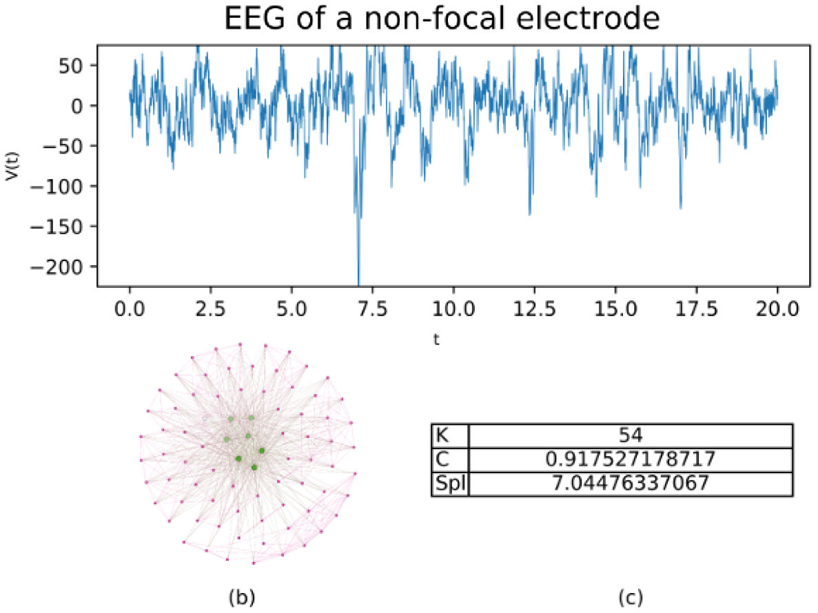
In Figs. 1 and 2, the Feigenbaum network is shown, along with the values of the parameters, average degree (K), average clustering (C), and average shortest path length (SPL) for two samples of 20 seconds type “F” and type “N” respectively.
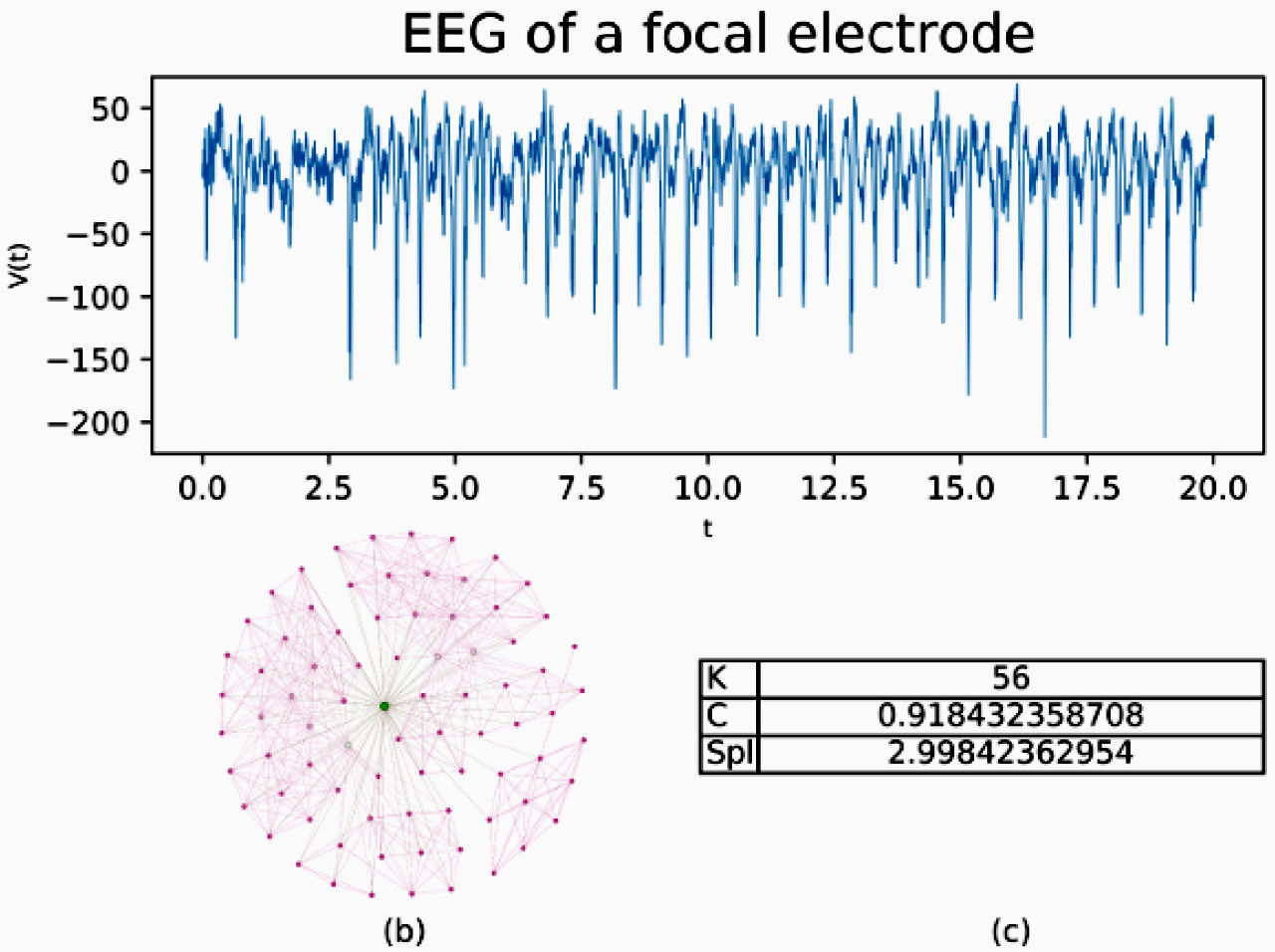
FIGURE 1 20 seconds of EEG activity from a focal electrode. b) shows a subnetwork for the EEG built by Feigenbaum approach, c) shows the values for average degree (K), average clustering (C) and average shortest path length (SPL).
2. EEG signals
The Data used was taken from the publicly available source of the Bern-Barcelona EEG database [37], where Andrzejak et al. originally made a correlation study.
The data were taken from intracranial EEG from five different epileptic patients. The EEG recordings were made as part of the diagnostics of the epileptic patients, prior and independently to this study. The EEG signals were either sampled at 512 or 1024 Hz, depending on whether it was a more or less than 64 channel record.
Each signal was filtered by a band-pass fourth-order Butterworth filter, between 0.5 and 150 Hz. Signals that were sampled at 1024 Hz, were down-sampled to 512 Hz.
Data were compiled into two different data sets: the “F” set, are the data from the focal epileptic point, which was identified as the first electrode that measures the epileptic seizure. And the “N” set, are the data from the non-focal points. A non-focal point is any other point that didn’t show the epileptic seizure.
Each data set was assembled by randomly selecting 7500 signals from a pool of 10240 samples, these samples were obtained by making windows of 20 seconds each. Recordings of seizure activity and three hours after were excluded from the data set. Before being included in the database, the signal was visually inspected to ensure non-significant artifacts were present. No clinical selection criterion, such as the presence or absence of epileptiform activity were applied.
3. Theory
Graph Theory has been used to study both the static and dynamic descriptions of complex systems. The “particles” or individual elements of the system are represented as nodes in the network and the interactions or links between these elements correspond to lines that join the nodes in pairs. The topology of these abstract objects allows to characterize certain types of network (small world, free scale, etc.) and associate them with some typical systems. The topology is determined by the number of links each node possesses (degree distribution), the clustering coefficient, or the average shortest path length between any pair of nodes. A comprehensive review of the subject can be found at http://networksciencebook.com/ [38].
3.1. Feigenbaum graphs
The Feigenbaum graphs are a tool that has been employed in the characterization time series data. By constructing a network from a given time series data set [39-41], the network structure extracts important information from said time series [42-46].
To characterize the data sets and achieve a systematic method for identifying epileptic focal points, each signal from the corresponding data set, “N” or “F”, was transformed into a Feigenbaum graph. Following the idea that most of the characteristics of the signals are translated to the topology of the network, the analysis of this topology is relevant.
The process for building the network is as follows: For each point x i in the data set, a node i is added to the network. Then, for each pair of points x i and x j in the set, every time the criterion x i ,x j > x n for all n, such that i < n < j is met, an edge is added between nodes i and j [12,44].
Following the aforementioned procedure for the example data in Fig. 3a), the network from Fig. 3b) is built. By building the Feigenbaum network a new structure is met for the data, and so it can be analyzed as such.
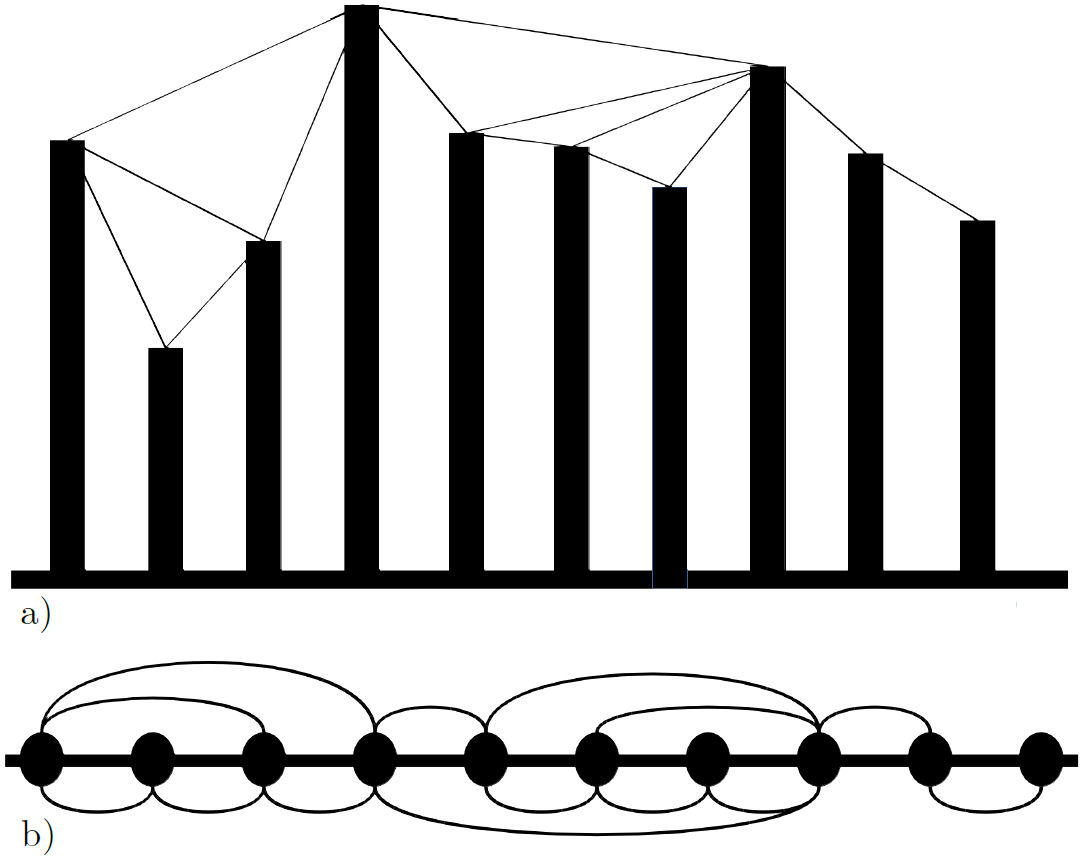
FIGURE 3 a) A data set where the lines indicate a link in the network. b) The network that results from the data in a), by following the mentioned procedure.
Take the EEG from Fig. 4a). For each data point, a node is added to the network in Fig. 4b), and the edges are created following the procedure in Figs. 3a) and Fig. 3b).
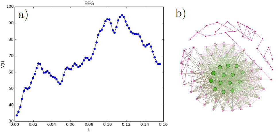
FIGURE 4 a) EEG data from the [37] data set. b) The network that results from the data in a), by following the mentioned procedure.
3.2. Statistical measurements
Once the Feigenbaum graphs were built, an analysis of the structure of the graphs is in order. To find a measure to characterize them as “N” or “F” whichever was the case, some calculations on the topology of the networks are of use.
To this end, we calculated the average shortest path length for each graph, as it has a direct correlation to the size of the graph, and the data itself. On the other hand, we calculated the average clustering coefficient. It is a measurement of how the network is connected and correlates with how auto-similar the data are.
Getting the average clustering coefficient for each network, a single number is set to identify each of the time windows in the data sets. Also by calculating the average shortest path length for each network, a new single number is obtained to identify each EEG signal of 20 seconds.
The average clustering coefficient is calculated in the simple form (1) [47].
where n is the number of nodes in the network G, and c v is the clustering coefficient for each node v.
The clustering coefficient c v is calculated using Eq. (2) [49].
where T(v) is the number of triangles through node v, and k(v) is the degree of v.
So the average shortest path length is calculated employing the Eq. (3) [50].
Where V is the set of nodes in the graph, d(s,t) is the shortest path length from s to t. And n is the number of nodes in the graph.
Because the average shortest path length and the average clustering coefficient of each graph are calculated, each signal in each data set gets identified by two singular numbers. As these numbers on their own are not singularly defining, a statistical approach must be made. For this end, each individual set of parameters were assembled in distributions for said parameter and data set, as shown in Figs. 5a), 6a), 5a) and 6b).
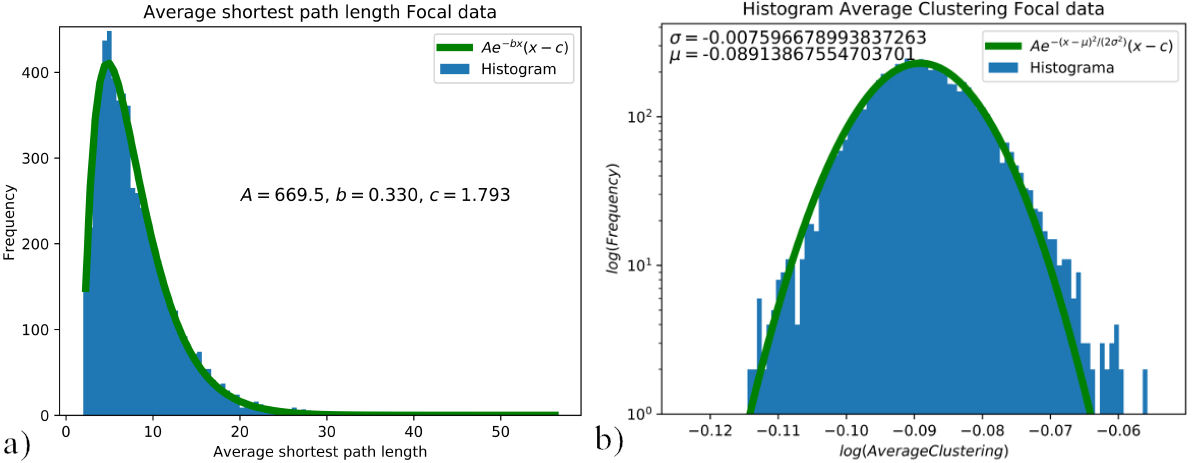
FIGURE 5 a) Distribution of the shortest path length for the focal data set, curve fitted to Aexp(−bx)(x − c) where A = 669.5, b = 0.330 and c = 1.793. b) Average clustering distribution for the focal data set, curve fitted to A exp(−(x − µ)2 /(2σ 2)), where σ = −0.007 and µ = −0.089. Distributions of average shortest path length 5a) and average clustering coefficient 5b) for focal data.
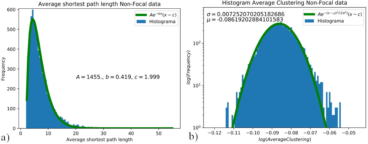
FIGURE 6 a) Distribution of the shortest path length for the nonfocal data set, curve fitted to Aexp(−bx)(x−c) where A = 1455, b = 0.419 and c = 1.999. b) Average clustering distribution for the non-focal data set, curve fitted to Aexp(−(x − µ)2 /(2σ 2)), where σ = −0.007 and µ = −0.086. Distributions of average shortest path length 6a), and average clustering coefficient 6b) for non-focal data.
4. Results and discussion
As every signal is processed, the parameters for the average shortest path length, and average clustering coefficient, are calculated and placed on their respective distribution.
The distribution for the average clustering coefficient was assembled for each data set; hence, one distribution for the EEG signals in the focal set “F”, and one for the EEG signal in the non-focal set “N”. These distributions were curve fitted to identify the difference or lack of between data sets. For the average clustering coefficient, the histogram is presented in the log scale and fitted to Aexp(−(x − µ)2 /(2σ 2)), as shown in Figs. 5b) and 6b). The tails on the average clustering coefficient distributions are not accounted for, without affecting the criteria for differentiation between focal and non-focal data. For the average shortest path length, the histogram is curve fitted to Aexp(−bx)(x − c), as shown in Fig. 5a) and 6a).
In order to increase statistical accuracy and significance 20 subsets of 2000 signals were built from the original 7500 signal data set, for both “N” and “F” signals. These sets were assembled by the same means of randomly selecting the 2000 signals from the pool. For these new 20 sets of signals, the distributions of average clustering coefficient and average shortest path length were assembled and fitted, as shown in Figs. 7a) and 7b).
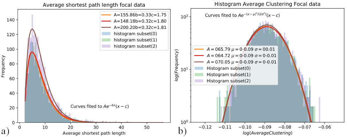
FIGURE 7 a) Distributions of the shortest path length, curve fitted to Aexp(−bx)(x − c), b) Average clustering distributions, curve fitted to Aexp(−(x − µ)2 /(2σ 2)). Distributions of average shortest path length 7a), and average clustering coefficient 7b) for 3 subsets of 2000 samples of focal data.
From the curve fitting of each new data subset, the relevant fitting parameters are established. The b parameter from the Aexp(−bx)(x−c) fit for the average shortest path length, is a way of characterizing both sets of data “N” and “F”. A comparison for this parameter is shown in Fig. 9a). The µ parameter from the Aexp(−(x − µ)2 /(2σ 2)) fit for the av- Parameters b and µ are chosen since they have the biggest erage clustering coefficient is also a way of differentiating weight in each curve fitting. As the data is assumed to have between both data sets “N” and “F” as shown in Fig. 9b). different structures for the focal “F” and non-focal “N” data, these parameters are the most important. Furthermore, the other parameters are non-significant to make any decisions if the data comes from focal or non-focal EEG, as shown in the plots for the σ, A, and c parameters in Fig. 8.
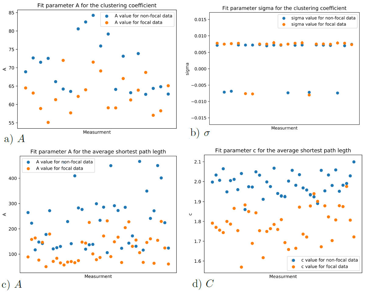
FIGURE 8 Fitting parameters for the average clustering coefficient and average shortest path length distributions.
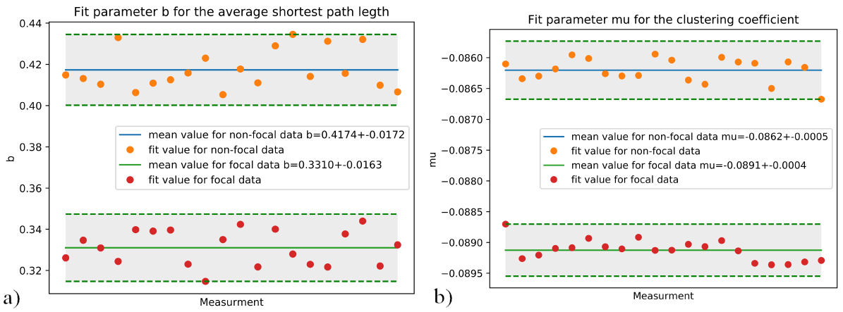
FIGURE 9 a) Comparison of the value of the b parameter for “N” and “F” data. b) Comparison of the µ parameter for “N” and “F” data. Relevant fitting parameters for Average clustering coefficient 9a) and average shortest path length 9b), 20 distributions of 2000 samples.
Following the same process, another 20 subsets of 1000 signals were built, for both “N” and “F” signals. The calculations of the average shortest path length and average clustering coefficient for these subsets were also assembled in distributions and fitted. The comparison of relevant fitting parameters, b for the average shortest path length in Fig. 10a) and µ for the clustering coefficient in Fig. 10b) are shown.
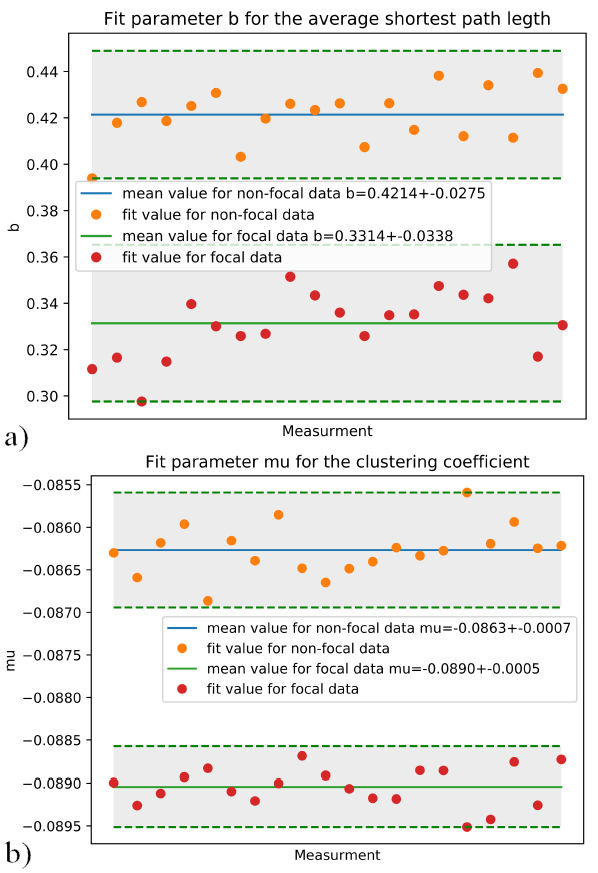
FIGURE 10 a) Comparison of the b parameter for “N” and “F” data. b) Comparison of the µ parameter for “N” and “F” data. Relevant fitting parameters for Average clustering coefficient 10a) and average shortest path length 10b), 20 distributions of 1000 samples.
In Table I, the values to differentiate between focal and non-focal data are presented. For the curve fitting of the average clustering coefficient Aexp(−bx)(x − c) the parameter b. And the parameter µ for the curve fit Aexp(−(x − µ)2 /(2σ 2)) of the average shortest path length. The differences shown in Table I are consistent when calculating for the entire data of 75000 samples, where b = 0.419 for nonfocal data and b = 0.330 for focal data, and µ = −0.089 for focal data and µ = 0.086 for non-focal data.
TABLE I Values of b and µ for focal and non-focal data.
| µ | b | |
| Focal data 2000 samples |
−0.0891±0.0004 | 0.3310±0.0163 |
| Non-focal data 2000 samples |
−0.0862±0.0005 | 0.4174±0.0172 |
| Focal data 1000 samples |
−0.0890±0.0005 | 0.3314±0.0338 |
| Non-focal data 1000 samples |
−0.0863±0.0007 | 0.4214±0.0275 |
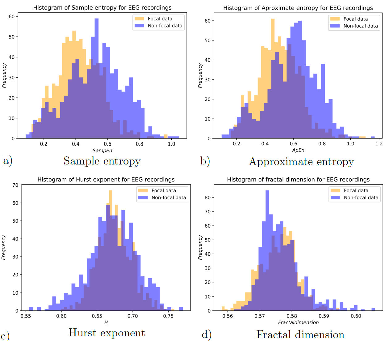
As a way to measure the effectiveness of these results, complementary measurements were made. The Hurst exponent, sample entropy approximate entropy and fractal dimension of the EEG recordings were calculated. Distributions for each of these measurements are shown in Fig. 11, for both focal and non-focal EEG data.
The usefulness of these measurements to differentiate each individual set of EEG recordings is estimated by means of the Kolmogorov-Smirnov (KS) statistic test. The results for the KS tests are presented in Table II, where one can see the statistical significance of each property of the EEG.
TABLE II KS-test results for different measurements
| ks statistic | P value | |
| Fit parameter b for spl | 1.0 | 0 |
| Fit parameter µ for C | 1.0 | 0 |
| For 2000 sample data sets |
||
| Fit parameter b for spl | 1.0 | 1.4508e−11 |
| Fit parameter µ for C | 1.0 | 1.4508e−11 |
| For 1000 sample data sets |
||
| Fit parameter b for spl | 1.0 | 1.4508e−11 |
| Fit parameter µ for C | 1.0 | 1.4508e−11 |
| Sample entropy | 0.30597 | 1.26894e-33 |
| Approximate entropy | 0.28731 | 1.21786e-29 |
| Hurst exponent | 0.10199 | 4.62265e-4 |
| Fractal dimension | 0.09577 | 1.24584e-3 |
5. Conclusion
In this work, a new method is proposed to identify epileptic focal zones from the Andrzejak et al. database [37]. It is managed by assembling Feigenbaum graphs and calculating distributions for the average shortest path length and average clustering coefficient from every data set. Fitting the average clustering coefficient to Aexp(−(x − µ)2 /(2σ 2)) and observing the µ parameter, if µ = −0.089±0.0005 the data is said to be focal, also if µ = −0.0863±0.0007 the data is said to be non-focal. This yields a differentiating factor between both focal and non-focal signals.
For the average shortest path length, the distribution, curve fitting to Aexp(−bx)(x − c) and checking for the b parameter. If b = 0.4214 ± 0.0275, the data are said to be non-focal, and if b = 0.3314±0.0338, the data are said to be focal, giving another criterion to differentiate between focal and non-focal signals.
As shown in Table I, this new approach yields better confidence to differentiate between focal and non-focal EEG. For the KS test, the b parameter and µ parameter can be used with a p-value of 0 and KS- statistic value of 1, hence is a much better differentiating factor than either of the Approximate entropy, Sample entropy, Hurst exponent, or fractal dimension factors.
Following the idea and how the data set are assembled, this measurement could be calculated for a single patient by assembling a data set created from segments -time windows of EEG studies no matter the timeline, and analyzing each signal. The calculation of the curve fit for the average shortest path length distribution, and the average clustering coefficient of the Feigenbaum graphs of the data set can be used to identify the focal EEG electrode readings.
Because the results are less scattered for the 2000 sample set than the 1000 sample set, it suggests that 2000 samples should be used for better results, although 1000 samples can be used at a lesser computational cost, since the KS-test values are the same for both sample sizes, KS − statistic = 1, and p − value = 1.4508e −11. This could help the physician assess a better diagnosis for the patient in the determination of epilepsy focal sites.
Subject to considering other databases and other probably more complex cases, we see that, with this technique, it is possible to distinguish between the signal that comes from an epileptic focus and another that does not, which can be of great value both in diagnosis and in the practical determination of focal sites for surgical intervention.


 nueva página del texto (beta)

