


 nueva página del texto (beta)
 Inglés (pdf)
 Artículo en XML
 Referencias del artículo
 Enviar artículo por email
 Citado por SciELO
  Similares en
SciELO
Similares en
SciELO 
 Permalink
1.Introduction
In the last decade, fractional differential equations played a very important role in the advancement of science and engineering. One of the most interesting fractional differential equations, utilized in physics, astrophysics, engineering, and chemistry, is the Lane-Emden (and Emden-Fowler) equation. Many methods were proposed to solve these equations. The fractional polytropic models were investigated by El-Nabulsi (2011) for white dwarf stars, Bayin and Krisch (2015) for the incompressible gas sphere, Abdel-Salam and Nouh (2016) and Yousif et al. (2021) for the isothermal gas sphere. Analytical solutions to the fractional Lane-Emden equations using series expansion and Adomian decomposition methods were introduced by Nouh and Abdel-Salam (2018a), Abdel-Salam and Nouh (2020), Nouh and Abdel-Salam (2018b), and Abdel-Salam et al. (2020).
Artificial Neural Networks (ANNs) have proved to be a very promising tool that has been used in wide areas of scientific research and has found many applications to solve problems related to geophysics, engineering, environmental sciences, and astronomy [e.g., Weaver (2000), Tagliaferri et al. (1999), Tagliaferri and Longo (2003), Faris et al. (2014), Elminir et al. (2007), El-Mallawany et al. (2014), Leshno et al. (1993), Lippmann (1989), Zhang (2000)]. The great potential of ANNs is the high-speed processing provided by their massive parallel implementations (Izeboudjen et al. 2014). Nowadays, ANNs are mostly used for universal function approximation in numerical paradigms because of their excellent properties of self-learning, adaptability, fault tolerance, nonlinearity, and advancement in input to output mapping (Wang et al. 2018). In addition, ANNs are effective, efficient and successful in providing a high level of capability to handle complex and noncomplex problems in many spheres of life. Besides, ANNs are appropriate for modeling many physical phenomena and have been used widely to solve fractional and integer differential equations problems with different patterns for the ANN architecture [Raja et al. (2010), Raja et al. (2011), Raja et al. (2015), Hadian-Rasanan et al. (2020), Pakdaman et al. (2017), Zuniga-Aguilar et al. (2017)]. In addition, Ahmad et al. (2017) used artificial neural networks (ANNs) to compute the solution of Lane-Emden type equations. Recently, Nouh et al. (2020) presented a solution to the fractional polytropic gas sphere (first kind of the Lane-Emden equation); the results indicated that the ANN method is precise when compared with other methods.
In the current work, we shall solve the fractional isothermal gas sphere equation using the Taylor series and train the ANN algorithm by using tables of the fractional Emden functions, mass-radius relations, and density profiles. For the sake of computational simulation, the normal feed-forward neural network is used to approximate the fractional Emden function solution, mass-radius relations, and density distributions which are in good agreement with other analytical schemes. The architecture used in this research is a feed-forward neural network that has three-layers and is trained using the back-propagation algorithm based on the gradient descent rule.
The rest of the paper is organized as follows: § 2 is devoted to the definition of the conformable fractional derivative. § 3 deals with the Taylor expansion solution of the fractional isothermal gas sphere equation. The mathematical modeling of the neural network is performed in § 4. In § 5, the results are introduced with discussions. The conclusion reached is given in § 5.
2.Conformable Fractional Derivative
Khalil et al. (2014) introduced the conformable fractional derivative using the limits in the form:
Here f α(0) is not defined. This fractional derivative reduces to the ordinary derivative when α = 1. The following properties are found for the conformable fractional derivative:
where f, g are two α-differentiable functions and c is an arbitrary constant. Equations (4) to (6) are demonstrated by (Khalil et al., 2014). The corresponding fractional derivative of certain functions could be given by:
3.Taylor Expansion of the Fractional Isothermal Gas Sphere Equation
Let us consider the isothermal equation of state given by
where K is the pressure constant. By implementing the principles of the conformable derivatives, Yousif et al. (2021) derived the conformable second-order nonlinear differential equation that describes the isothermal gas sphere as
The mass contained in the sphere is given by
the radius is given by
where
Equation (9) can be written as
The fractional Taylor series solution for any function u(x) can be written as
Equation (13) can be written in the following form
Differentiating Equation (14) with respect to α, we get
Putting x = 0 in the last equation, we have
Differentiating equation (15) with respect to α, we get
When x = 0,we have
Differentiating Equation (16) with respect to α, we have
When x = 0 we have
and so on. Finally, we have
Thus the solution of Equation (13) is given by
4. Neural Network Algorithm
4.1.Mathematical Modeling of the Problem
The neural network architecture used to model the equation of conformal fractional isothermal gas spheres is shown in Figure 1. We write equation (9) as

Fig. 1 ANN Architecture developed to simulate the fractional isothermal Emden function, mass-radius relation, and density profiles.
Along with the initial conditions u(0) = 1 and
where A(x) fulfills the initial conditions and f(x, N(x,p)) indicates the feed-forward neural network, and N(x,p) is the output of the neural network. The vector x is the network input and p is the analogous vector of adaptable weight parameters. Then N(x,p) can be written as
where
the n th fractional derivative of N(x,p) gives
Then, the approximate solution is given by
This satisfies the initial conditions as:
and
so that
4.2.Gradient Computations and Parameter Updating
Assuming that Equation (23) represents the approximate solution, the problem will be turned into an unconstrained optimization problem and the amount of error will be given by
Here:
and
where
The conformable fractional derivative is considered at par with a feed-forward neural network N with one hidden layer for each of its inputs, with the same weight values w and thresholds β
i
with each weight v
i
being exchanged with v
i
P
i
where
The updating rule of the network parameters can be specified as
where α, b, c are learning rates, i = 1,2,…,n, and j = 1,2,…, h.
4.3.Back-Propagation Training Algorithm
The back-propagation (BP) training algorithm is a gradient algorithm aimed to minimize the average square error between the desired output and the actual output of a feed-forward network. Continuously differentiable non-linearity is required for this algorithm. The gradient algorithm mathematics must assure that a specific node has to be adapted in a direct rate to the error in the units it is connected to. This algorithm has been described in detail in our previous paper (Nouh et al. 2020). Figure 2 shows a flow chart of an off-line back-propagation training algorithm, see Nouh et al. (2020), Yadav et al. (2015).

The back-propagation (BP) learning algorithm is a recursive algorithm starting at the output units and working back to the first hidden layer. A comparison of the desired output t j with the actual output u j at the output layer is executed using an error function which has the following form:
The error function for the hidden layer takes the following form:
where δj is the error term of the output layer, and wk is the weight between the output and hidden layers. The update of the weight of each connection is implemented by replicating the error in a backward direction from the output layer to the input layer as follows:
The learning rate η is chosen such that it is neither too large leading to overshooting nor very small leading to a slow convergence rate. The last part in Equation (36) is the momentum term which is affixed with a constant γ (momentum) to accelerate the error convergence of the back-propagation learning algorithm, and also to assist in pushing the changes of the energy function over local increases and boosting the weights in the direction of the overall downhill, Denz (1998). This part is used to add a portion of the most recent weight values to the current weight values. The values of the η and γ terms are set at the beginning of the training phase and determine the network speed and stability, see Basheer and Hajmeer (2000).The process is repeated for each input pattern until the output error of the network is decreased to a pre-specified threshold value.
The final weight values are frozen and utilized to get the precise values of the desired output during the test phase. The quality and success of training of ANN are assessed by calculating the error for the whole batch of training patterns using the normalized RMS error that is defined as:
where J is the number of output units, P is the number of training patterns, t pj is the desired output at unit j, and u pj is the actual output at the same unit j. A zero error denotes that all the output patterns computed by the isothermal gas spheres ANN perfectly match the values expected, and that the isothermal gas spheres ANN is fully trained. Similarly, internal unit thresholds are adjusted by supposing that they are connection weights on links from the input with an auxiliary constant-value.
5.Results and Discussions
5.1.Data Preparation
We developed a MATHEMATICA routine to calculate the fractional Emden function and the physical characteristics of the conformable isothermal gas spheres, like mass (equation 10), radius (equation 11), and density (equation 12). Equation (17) represents the series solution of fractional isothermal gas spheres, which is similar to the power series solution developed by Yousif et al. (2020), where we used only 10 series terms. As pointed out by Yousif et al. (2020), this series expansion (like equation 17) diverges for x >3.2. We used the accelerated scheme developed by Nouh (2004) to accelerate the series. Our calculations are done for a range of fractional parameters (0.75 ≤ α ≤ 1) with a step of 0.1. For the integer case (α = 1), the Emden function computed according to the series solution, and the numerical one, are in good agreement, Yousif et al. (2021). Fractional models for the isothermal gas sphere can be computed using Equations (10) to (12) for the mass, radius, and density. So, we can investigate the mass-radius relations and density profiles at different fractional parameters.
In Table 1, we list the mass-radius relations for some fractional isothermal gas spheres models. The designations in the table are: R* and M* represent the radius and mass of the fractional star, R0 and M0 are the radius and mass of a typical neutron star with the physical parameters
5.2.Network Training
To train the proposed neural network used to simulate the conformable fractional isothermal gas sphere equation, we used data calculated in the previous subsection. The data used for training of the ANN are shown in the first column of Tables (2-3).
Table 2. Training, validation, and testing data for the fractional isothermal Emden function.
| Training phase | Validation phase | Testing phase |
| α | α | α |
| 0.8, 0.85, 0.9, | 0.96, 0.99 | 0.91, 0.92, |
| 0.95, 0.97, 0.98, 1 | 0.93, 0.94 |
Table 3. Training, validation, and testing data for mass-radius relations and density profiles.
| Training phase | Validation phase | Testing phase |
| α | α | α |
| 0.75, 0.90, 0.92, | 0.95, 0.98 | 0.80, 0.85, 0.91 |
| 0.93, 0.94, 0.96, | ||
| 0.97, 0.99 |
The architecture of the neural network (NN) we used in this paper for the isothermal gas sphere function is 2-120-1, where the input layer has two inputs, which are the fractional parameter α and the dimensionless parameter x (xtakes values from 0 to 80 in steps of 0.1), while the output layer has 1 node for the isothermal gas sphere function u computed for the same values of the dimensionless parameter x and input fractional parameter α. For the mass-radius relation, we used the architecture 2-120-2, where the input layer has two individual inputs, which are the fractional parameter α and the radius of the star R, while the output layer has 2 nodes, which are the mass and density at the same values of the input fractional parameters.
The choice of 120 neurons in the hidden layer of the NN was decided according to the findings we reached in our previous research (Nouh et al., 2020) after testing 80,120 and 200 neurons in one hidden layer of NN (shown in Figure 1), which gave the least RMS error and the best model for the network compared to the other two configurations for both the isothermal and mass-radius relation cases.
After multiple modifications and adjustments to the parameters of the NN, it converged to an RMS error value of 0.00002 for the training of the isothermal case, and to a value of 0.000025 for the training of the mass-radius relation and density profile case. During the raining of the NN, we used a value for the learning rate (α =0.03) and for the momentum (α = 0.5). These values for the learning rate and momentum proved to quicken the convergence of the back-propagation training phase without exceeding the solution. In this research, we have programmed our algorithms using the C++ programming language running on Windows 7 of a CORE i7 PC. The network training typically took around 3 hrs. to converge for each case of the training previously mentioned. The trainings were implemented concurrently on different windows of the same machine. After network training, the frozen saved weights were utilized to get the values of the desired output during the validation and test phases in a very short time (about 1 second), as described in the next section.
For the demonstration of the convergence and stability of the values computed for the weight parameters of the network layers the behavior of the convergence of the input layer weights, bias and output layer weights (wi, β i and v i ) for the isothermal gas sphere case is as displayed in Figure 3. Moreover, the convergence behavior and stability of the values computed for the weight parameters of network layers (weights of the input layer, bias, and output layer) for the mass-radius relation case are shown in Figure 4. As these figures indicate, the values of the weights were initialized to random values and after many iterations they converged to stable values.

Fig. 3 Convergence of input, bias, and output weights for the fractional isothermal Emden function. The color figure can be viewed online.

5.3.Validation and Test of the Training Phase
To ensure the training of the NN, we used two values for the fractional parameter α, not being used in the training phase as a validation and verification of the goodness of that phase. These two values are shown in the middle column of Table 2 and Table 3 for the isothermal Emden function, and mass-radius relations and density profiles cases, respectively. The obtained results for those two validation values are as shown in Figure 5 for the isothermal Emden function, in Figure 7 for the fractional density profiles, and in Figure 9 for the fractional mass-radius relations. As shown in these figures, there is a very good coincidence between the NN prediction and the analytical results for the Emden function, mass-radius relations, and density profiles, where the maximum absolute error is 1%, 2.5% and 4%, respectively. We plotted the analytical solution and the NN prediction for the Emden function and the density profile with different colors, but due to the overlapping of the two curves, they appear as one. The big difference comes from the region near the center of the sphere, for x ≤ 10. In the case of the mass-radius relation (Figure 9), the noticeable difference between the analytical solution and the NN is larger than that of the Emden function and density profiles due to the nature of the equation relating the mass to the radius (equation 10).

Fig. 5 The fractional Emden functions of the isothermal gas sphere obtained in the validation phase. The analytical and the ANN solutions are plotted with different colors. The maximum relative error is 1%. The color figure can be viewed online.
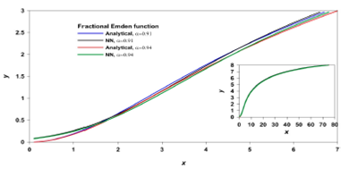
Fig. 6. Thefractional Emden functions of the isothermal gas sphere obtained in the test phase. We plot the analytical and the corresponding ANN solutions with different colors to show the accuracy of the calculations. Also, the complete curve is included in the graph. The color figure can be viewed online.
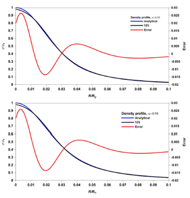
Fig. 7 The fractional density profiles obtained in the validation phase. There is a very low error except for the range of the radius ratio R/R0 ≤ 0.015. The maximum relative error is 2.5%. The color figure can be viewed online.

Fig. 8 The fractional density profiles obtained in the test phase for the fractional parameters a = 0.8,0.85.The color figure can be viewed online.

Fig. 9 The fractional mass-radius relations obtained in the validation phase. The maximum relative error is 4%. The color figure can be viewed online.
In Figures (6), (8), and (10), we plotted the predicted values of Emden functions, density profiles and mass-radius relations for some values of the fractional parameters listed in Tables 1 and 2. In these figures, due to the small change of the Emden function and density with the fractional parameter, and also the negligible difference between the analytical solution and the NN solution, we truncated the x-axis at a smaller value for more clarity. Again, there is a somewhat noticeable difference between the analytical solution and the predicted NN values in the case of the mass-radius relation (Figure 10) which is larger than the other two predicted NN values for the Emden functions and the density profiles (Figure 6 and Figure 8). This large difference may be attributed to the instability during performing and accelerating the series expansion of the fractional derivative of the Emden function (equation 10). It should be noted, here again, that the time taken to get the results of the validation and test phases, using the frozen saved values of the weights of the trained NN, is negligible (around 1 second). This proves the high efficiency and high-speed processing of the ANN when compared with the numerical and analytical methods.

6.Conclusion
The ANN modeling of the nonlinear differential equations shows a high efficiency when compared with the numerical and analytical methods. In the present work, we aimed to introduce a computational approach to the fractional isothermal gas sphere via ANN. We solved the second type of Lane-Emden equation (the isothermal gas sphere) using the Taylor series, then we accelerated the resulting series to reach a good accuracy. The analytical calculations are performed for the Emden functions, mass-radius relations, and density profiles.
We obtained a good accuracy through the use of the ANN technique by using some calculated data to train the NN in the training phase, then validating the trained network by some other values, where we obtained maximum error values of 1%, 2.5% and for the isothermal fractional Emden function case, the density profile case, and the mass-radius relation case, respectively. To test the ANN technique in predicting unknown values, we used the trained network and ran the routine for the fractional test parameters listed in Tables 2 and 3. The comparison between the analytical and the ANN solution gives a very good agreement, as shown in Figures (6, 8, and 10) with a maximum error of 4%. The results obtained reflect the applicability and efficiency of using ANN to model stellar physical characteristics (i.e., radius, mass, and density) using the fractional isothermal gas sphere. In our opinion, the present results, besides the results obtained in Nouh et al. (2020), are an important step toward the composite modeling (e.g., isothermal core and polytropic envelope) of various stellar configurations using ANN.

