


 nueva página del texto (beta)
 Inglés (pdf)
 Artículo en XML
 Referencias del artículo
 Enviar artículo por email
 Citado por SciELO
  Similares en
SciELO
Similares en
SciELO 
 Permalink
Introduction
Almost 50% of the ocean floor is covered by calcareous material, 14% by siliceous material and the rest by clays (Seibold and Berger 1996). Coccoliths and foraminifera are the main planktonic components of the calcareous material (Haq and Boersma 1998, Abrantes et al. 2002, Bárcena et al. 2004). Coccolithophores (class: Prymnesiophyceae) are unicellular protists, smaller than 20 μm, that are covered by small plates of calcium carbonate called coccoliths (Brand 1994); they are among the main components of marine phytoplankton and have a worldwide distribution (McIntyre and Bé 1967, Okada and Honjo 1973). Foraminifera (class: Rhizaria), however, are unicellular protozoa (Simpson and Roger 2004) capable of producing a shell of calcium carbonate, also called a “test,” or of agglutinated particles (Loeblich et al. 1957). In both groups, the morphology of the calcareous structures is of paramount importance for individual taxonomic classification (Abrantes et al. 2002, Bárcena et al. 2004, Engel et al. 2009). The ecological composition and distribution patterns of coccolithophores and foraminifera are largely determined by climatic and hydrographic conditions, such as water masses and particularly temperature and salinity, making them a useful tool for paleoenvironmental and paleoceanographic studies (Barker and Berggren 1977, Lipps et al. 1979, Beckmann et al. 1981).
Much of the knowledge about the composition and fluxes of these organisms has been gained from time-series studies on sediment traps (Abrantes et al. 2002, Bárcena et al. 2004), where estimates indicate that coccolithophores can constitute up to 55% of total CaCO3 (Broerse et al. 2000) and that planktonic foraminifera contribute between 23% and 55% of the total flux of calcite (Schiebel 2002). However, most of these studies have been carried out in open oceanic areas, where oceanographic conditions show little variability. Ocean dynamics in coastal zones are more complex due to the processes involved therein, such as sediment input by lateral advection, resuspension of material, and coastal upwelling. Since there is not enough information on the fluxes of these groups of calcareous plankton for this area, the main objective of this work is to document the composition and magnitude of the fluxes of coccolithophores and foraminifera and to estimate their CaCO3 contribution in a sediment trap installed at 300 m depth off the coast of Ensenada, Baja California (Mexico), from April 1 to October 15, 2012.
Materials and methods
Oceanographic conditions
The study area is located within the southern limit of the California Current System, where oceanographic features are those typical of an eastern border circulation system because of the coastal upwelling events, which occur with maximum intensity in spring-summer and with a predominant flow towards the equator (Gómez-Valdés 1983, Lynn and Simpson 1987, Durazo et al. 2010). In this zone there is confluence of Subarctic Water, which is transported southward by the California Current; Tropical Surface Water and Tropical Subsurface Water, which are transported from the south and southwestern areas off the Baja California Peninsula (Lynn and Simpson 1987); and the California Countercurrent, which carries Equatorial Subsurface Water below 400 m and has a poleward flow (Durazo and Baumgartner 2002). The variability of the coastal upwelling index (CUI) showed a minimum value of 50 m3·s-1 per 100 m of coastline in February and a maximum of 250 m3·s-1 per 100 m of coastline in June (Fig. 1). Sea surface temperature fluctuated from 14 ºC in April to 22 ºC in September. Net primary productivity ranged from 900 mg C·m-2·d-1 in September to a maximum of 7,000 mg C·m-2·d-1 in March.
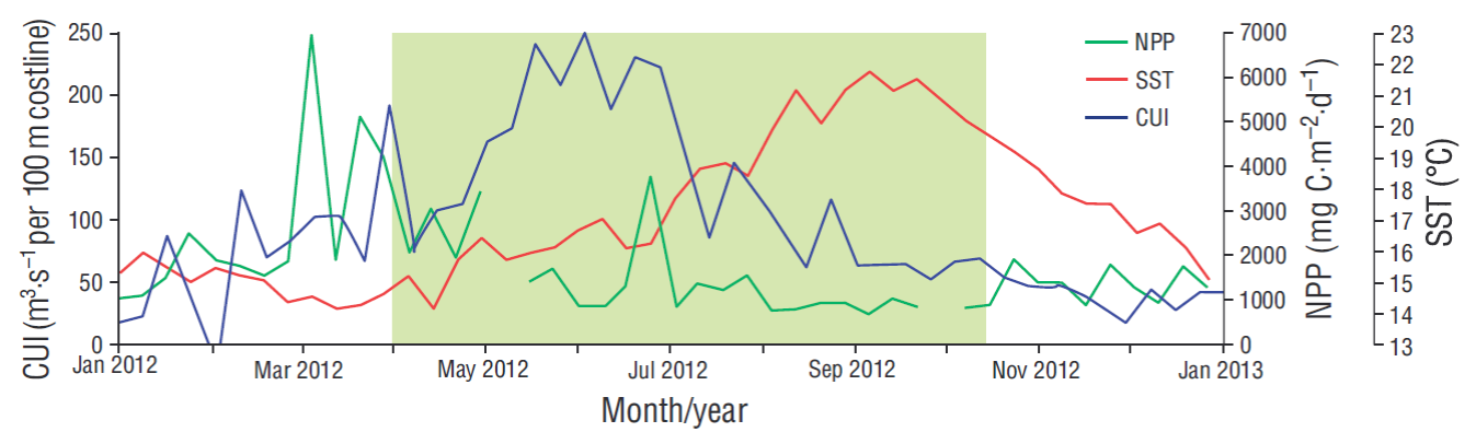
Figure 1 Variability of the coastal upwelling index (CUI, m3·s-1 per 100 m of coastline; available from http://www.pfeg.noaa.gov/products/PFEL/modeled/indices/upwelling/NA/data_download.html), net primary productivity (NPP, available from http://orca.science. oregonstate.edu/1080.by.2160.8day.hdf.mld.hycom.php), and sea surface temperature (SST, available from https://oceancolor.gsfc.nasa. gov/cgi/l3) in 2012. The green rectangle highlights the study period.
Sampling
The sediment trap (Technicap, PPS 3/3 with an opening area of 0.125 m2) was installed at 300 m depth off the coast of Ensenada, Baja California (Mexico) (31º45ʹ27ʺN and 116º39ʹ53ʺW). This area is known as the “Todos Santos Canyon” (Fig. 2). The time resolution for each sample was 17 days; the study period covered the time interval between 1 April and 15 October 2012 in order to document the influence of coastal upwelling events (with maximum intensity in spring-summer). The sediment trap had a carousel of 12 sampling bottles labeled A-1 to A-12. Each bottle contained a preserving solution, buffered with sodium tetraborate and 8.5 pH to avoid the dissolution of carbonates. A detailed description of the mooring and general treatment of the samples can be found in Silverberg et al. (2014). Eleven bottles were recovered from the sediment trap and 10 aliquots were obtained from each. One aliquot was used to analyze coccolithophores and another to analyze foraminifera. In both cases organic matter was eliminated according to Bairbakhish et al. (1999). For the coccolith analysis samples were filtered using Nucleopore membranes (47 mm diameter, 0.45 μm pore size). Part of the filter was mounted on aluminum supports and covered with 15 nm of platinum following the method described by Bollmann et al. (2002). A scanning electron microscope (Zeiss Supra 55VP) was used to digitalize 1,500 images (3,000× resolution) and analyze an area of 6.53 × 10⁻⁶ m2. Taxonomic identification of coccolithophores was done using the taxonomic identification concepts of Young et al. (2003) and the concepts of Quinn et al. (2005) for the Florisphaera profunda morphotypes, of Bollmann (1997) for Gephyrocapsa oceanica, and of Kleijne and Cros (2009) for the Syracosphaera group. The software Image-J was used to count coccoliths. After obtaining the number of coccoliths per sample and species, the flux of coccoliths was calculated following Andruleit (1997). Coccolith contribution to CaCO3 flux was estimated according to Young and Ziveri (2000).
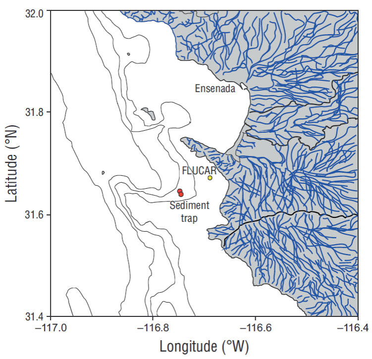
Figure 2 Location of the sediment trap (31º45ʹ27ʺN, 116º39ʹ53ʺW) (red circles), and the FLUCAR station (yellow circle). Blue lines show the drainage basins that channel to the sea.
Samples for the analysis of foraminifera were screened through a 63-μm mesh using distilled water (8.5 pH). Foraminifera were subsequently collected using a fine brush and a stereoscope. Identification was done according to Parker (1962), Boersma (1998), and Kemle-von-Mücke and Hemleben (1999). The flux of foraminifera is represented by the number of tests (shells) per square meter per day (tests·m-2·d-1), accounting for the number of tests, the times the sample was divided (split factor), the time during which the trap was collecting material, and the opening of the sediment trap (King and Howard 2001). All collected tests were then weighed per sample in an analytical microbalance (UMX2 Mettler Toledo, ± 0.001 mg accuracy) to obtain the weight of each sample in milligrams of calcite.
Inorganic carbon content was determined by analyzing 2 size fractions (<63 μm and >63 μm) with a CM5014 coulometer. The accuracy of the method was controlled by placing standard sediment (CM301-002) and performing 3 replicates of samples A-1, A-6, and A-11. Inorganic carbon (essentially in the form of CaCO3) was determined by calcu-lating the difference between total carbon and organic carbon content (unpublished data) (Ljutsarev 1987).
Results
Thirty-three species of coccoliths were taxonomically identified throughout the study period. The daily flux of coccoliths ranged from 27 × 106 coccoliths·m-2·d-1 in sample A-12 to 1,539 × 106 coccoliths·m-2·d-1 in sample A-8, with an average of 356 × 106 coccoliths·m-2·d-1 (Fig. 3a). No coccoliths were recorded from 25 August to 10 September 2012 (sample A-10). Emiliania huxleyi type A (huxleyi), E. huxleyi type B (pujosiae), G. oceanica morphotype Equatorial, and G. oceanica morphotype Larger accounted for 74% of the total flux of coccoliths. Calcidiscus leptoporus (larger), C. leptoporus (small), F. profunda var. elongata (medium), and Helicosphaera carteri accounted for 12% of the total flux of coccoliths, while the remaining 14% was contributed by other species.
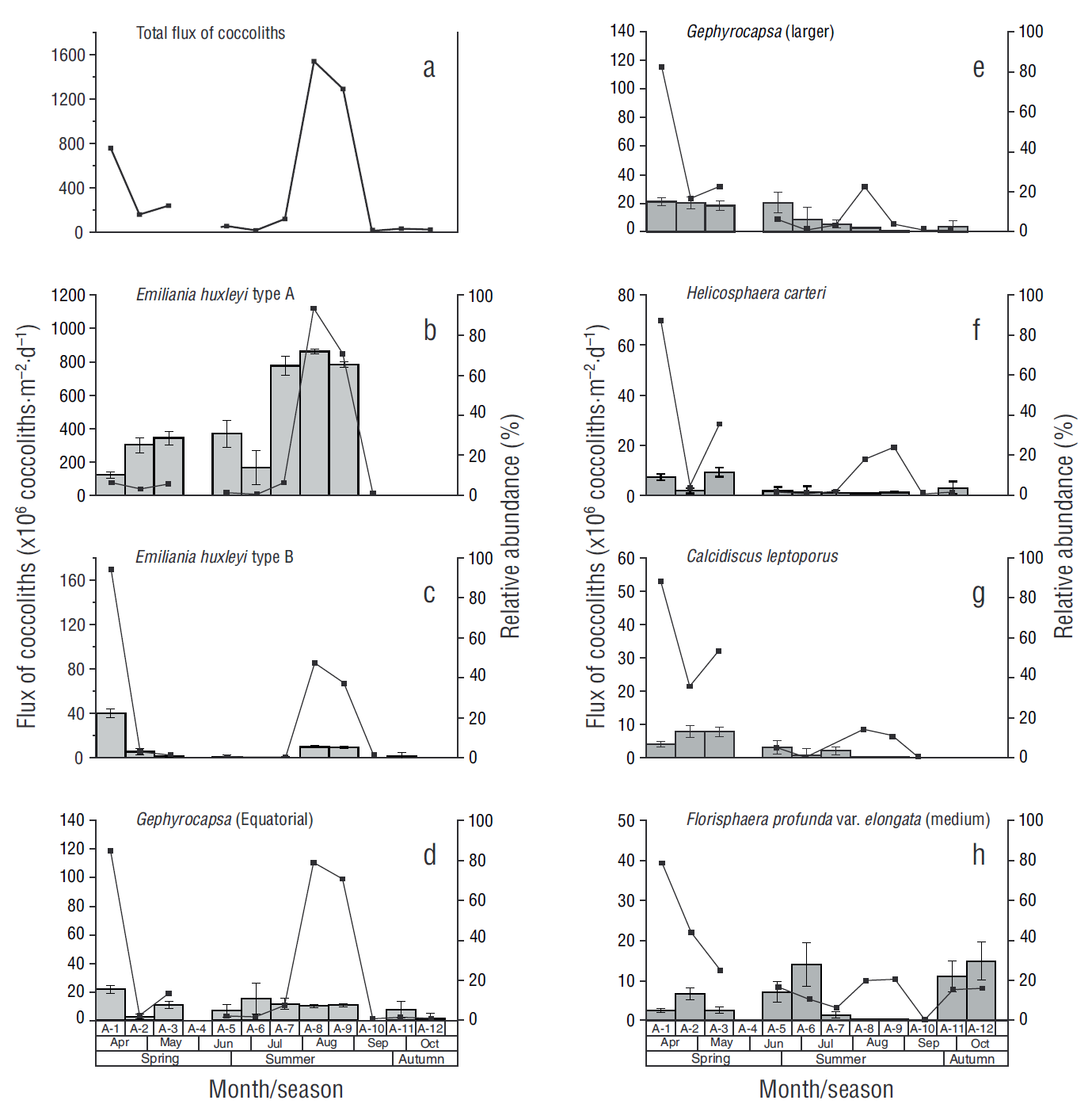
Figure 3 Flux of coccoliths (continuous line) and relative abundance (gray bars, SE at 95% confidence) in each sample (A-1-A-12). The total flux of coccoliths recorded during the study period and the fluxes of the most representative species are shown.
The fluxes of E. huxleyi type A varied from zero coccoliths in samples A-11 and A-12 to 1,114 × 106 coccoliths·m-2·d-1 in sample A-9, with an average of 188 × 106 coccoliths·m-2·d-1 and 73% maximum relative abundance (A-8) (Fig. 3b). The fluxes of E. huxleyi type B varied from zero coccoliths (A-6 and A-12) to 169 × 106 coccoliths·m-2·d-1 (A-1), with an average of 27 × 106 coccoliths·m-2·d-1 and 22% maximum relative abundance (A-1) (Fig. 3c). Gephyrocapsa oceanica morphotype Equatorial showed the second highest flux, ranging from 3 × 10⁶ coccoliths·m-2·d-1 in sample A-12 to 119 × 106 coccoliths·m-2·d-1 in sample A-1, with an average of 30 × 106 coccoliths·m-2·d-1 and 15.5% maximum relative abundance (A-1) (Fig. 3d). In the case of G. oceanica morphotype Larger, fluxes ranged from zero coccoliths in sample A-12 to 114 × 106 coccoliths·m-2·d-1 in sample A-1, with an average of 18 × 106 coccoliths·m-2·d-1 and 15% relative abundance (A-1) (Fig. 3e). Helicosphaera carteri reached a maximum flux of 69 × 106 coccoliths·m-2·d-1 in sample A-1, and a mean relative abundance of 11.6% in sample A-3 (Fig. 3f) Calcidiscus leptoporus showed a maximum flux of 53 × 106 coccoliths·m-2·d-1 in sample A-1 and a relative abundance of 13.2% in samples A-2 and A-3 (Fig. 3g). Lastly, F. profunda var. elongata (medium) showed a maximum flux of 39 × 106 coccoliths·m-2·d-1 in sample A-1 and a relative abundance of 29% in sample A-12 (Fig. 3h). Despite the low fluxes of species such as H. carteri and C. leptoporus, their contribution to CaCO3 content was high.
Estimation of coccolith contribution to total CaCO3 content showed maximum values in sample A-1 (25.4 mg·m-2·d-1) and minimum values in sample A-10 (0.0 mg·m-2·d-1). The coccolith species that most contributed to total CaCO3 content were H. carteri with 30% (10.0 mg·m-2·d-1) and C. leptoporus with 32% (8.7 mg·m-2·d-1). Gephyrocapsa oceanica mor-photype Equatorial reached a maximum contribution of 2.1 mg·m-2·d-1, which represents 10% of coccolith contribution to CaCO3 content. Contribution from E. huxleyi type A was 3.2 mg·m-2·d-1, which represents 10% of total contribution. Gephyrocapsa oceanica morphotype Larger contributed 3.0 mg·m-2·d-1, which represents 9% of the total contribution to CaCO3 content (Table 1).
Table 1 Estimation of coccolith contribution (mg CaCO3·m-2·d-1) to the flux of CaCO3 in each sample. Calcite estimations are based on the weights (pg) and sizes reported by Young and Ziveri (2000). The 6 species that contributed to a greater extent are shown. Species with low contributions are grouped into “Other species.”
| Sampling interval | Sample | Total CaCO3 | Calcidiscus leptoporus (Larger) | Helicosphaera carteri | Gephyrocapsa oceanica (medium) | Emiliania huxleyi huxleyi | Gephyrocapsa oceanica Larger | Calcidiscus leptoporus (small) | Others species | |
| Beginning | End | |||||||||
| 1 Apr 2012 | 10 Apr 2012 | A-1 | 25.4 | 8.7 | 10.0 | 2.1 | 0.2 | 3.0 | 0.3 | 1.1 |
| 11 Apr 2012 | 27 Apr 2012 | A-2 | 5.4 | 3.5 | 0.5 | 0.1 | 0.1 | 0.6 | 0.2 | 0.4 |
| 28 Apr 2012 | 14 May 2012 | A-3 | 11.1 | 5.3 | 4.0 | 0.3 | 0.2 | 0.8 | 0.3 | 0.2 |
| 15 May 2012 | 31 May 2012 | A-4 | ||||||||
| 1 Jun 2012 | 17 Jun 2012 | A-5 | 1.2 | 0.5 | 0.2 | 0.1 | 0.1 | 0.2 | 0.1 | 0.1 |
| 18 Jun 2012 | 4 Jul 2012 | A-6 | 0.2 | 0.1 | 0.0 | 0.0 | 0.0 | 0.0 | 0.0 | 0.1 |
| 5 Jul 2012 | 21 Jul 2012 | A-7 | 1.7 | 0.7 | 0.2 | 0.2 | 0.2 | 0.1 | 0.0 | 0.1 |
| 22 Jul 2012 | 7 Aug 2012 | A-8 | 11.2 | 1.4 | 2.1 | 2.0 | 3.2 | 0.8 | 0.6 | 1.0 |
| 8 Aug 2012 | 24 Aug 2012 | A-9 | 10.1 | 1.1 | 2.7 | 1.8 | 2.5 | 0.1 | 0.9 | 0.9 |
| 25 Aug 2012 | 10 Sep 2012 | A-10 | 0.0 | 0.0 | 0.0 | 0.0 | 0.0 | 0.0 | 0.0 | 0.0 |
| 11 Sep 2012 | 27 Sep 2012 | A-11 | 0.4 | 0.0 | 0.2 | 0.0 | 0.0 | 0.0 | 0.0 | 0.1 |
| 28 Sep 2012 | 14 Oct 2012 | A-12 | 0.1 | 0.0 | 0.0 | 0.0 | 0.0 | 0.0 | 0.0 | 0.1 |
In the case of foraminifera, 6 planktonic genera and 3 benthic genera were identified. All planktonic genera were identified in the <63 μm fraction. Globigerina spp. was the main contributor (50%), followed by Neogloboquadrina spp. (34%) and to a less extent Globorotalia spp. (6%), Pulleniatina spp. (5%), Globigerinoides spp. (3%), and Orbulina spp. (2%). Fluxes of planktonic foraminifera ranged from 9 tests·m-2·d-1 in samples A-2 and A-6 to 513 tests·m-2·d-1 in sample A-9, with an average of 137 tests·m-2·d-1 (Fig. 4a). The maximum fluxes recorded for these species are listed from highest to lowest: 249 tests·m-2·d-1 for Globigerina spp. (Fig. 4b), 103 tests·m-2·d-1 for Globorotalia spp. (Fig. 4c), 94 tests·m-2·d-1 for Neogloboquadrina spp. (Fig. 4d), and tests·m-2·d-1 for Globigerinoides spp. (Fig. 4e); all these fluxes were recorded in sample A-9. The maximum flux for Pulleniatina spp. and for Orbulina spp. was 9 tests·m-2·d-1 (Fig. 4f), but the latter was recorded only in sample A-11 (Fig. 4g). The most abundant benthic foraminifera were Quinqueloculina spp. (maximum of 212 tests·m-2·d-1, A-9), Textularia spp. (94 tests·m-2·d-1, A-1), and Bolivina spp. (40 tests·m-2·d-1, A-10). The species from these 3 genera rep-resented up to 50% of the CaCO3 contribution by planktonic and benthic foraminifera in certain samples (A-1, A-8, A-9, A-11, and A-12).
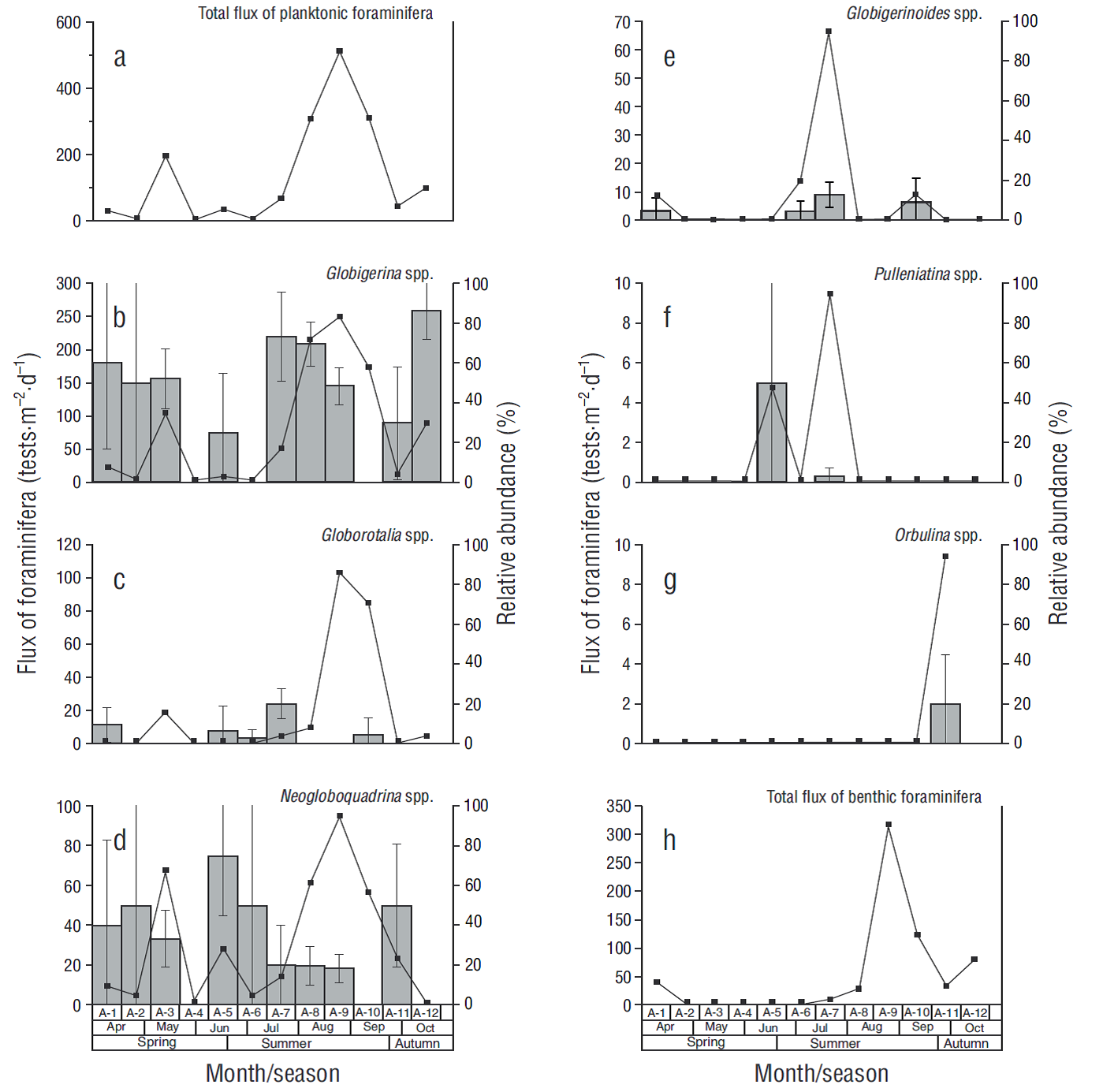
Figure 4 Flux of foraminifera (continuous line) and relative abundance (gray bars, SE at 95% confidence) in each sample (A-1 to A-12). The total flux of planktonic and benthic foraminifera (a, h) and the 2 most representative genera of planktonic foraminifera (b, c, d, e, f, g) are shown.
The CaCO3 concentrations determined by coulometry (>63 μm and <63 μm) showed a highly variable distribution. In the >63 μm fraction, fluxes varied from 18 mg·m-2·d-1 in sample A-8 to 490 mg·m-2·d-1 in sample A-2, with an overall average of 278 ± 170 mg·m-2·d-1. On the other hand, in the <63 μm fraction fluxes ranged from 46 mg·m-2·d-1 in sample A-6 to 356 mg·m-2·d-1 in sample A-2, with an average of 240 ± 144 mg·m-2·d-1 (Fig. 5a). The CaCO3 contribution from coccoliths reached a maximum of 25.4 mg·m-2·d-1 and was not consistent with the CaCO3 concentration measured by coulometry (Fig. 5b). Contribution of planktonic foraminifera to CaCO3 flux varied seasonally, with maximum fluxes of 0.07 and 0.62 mg·m-2·d-1 in samples A-12 and A-11, respectively, and an average of 0.25 mg·m-2·d-1 (Table 2, Fig. 5c). Benthic foraminifera contributed from 0.0 mg·m-2·d-1 in samples A-2, A-3, A-5, and A-6 to 0.8 mg·m-2·d-1 in sample A-1, with an average flux of 0.24 mg·m-2·d-1 (Table 3, Fig. 5d).
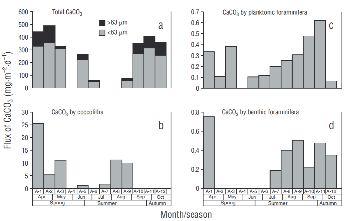
Figure 5 Total CaCO3 measured by coulometry for the 2 fractions analyzed (<63 μm and > 63 μm) (a) and CaCO3 supplied by coccoliths (b), planktonic foraminifera (c), and benthic foraminifera (d) in each sample (A-1 to A-12).
Table 2 Total flux of planktonic foraminifera, flux of CaCO3 (recorded in each sample), and relative abundance (RA, %) and flux of the identified genera (tests·m-2·d-1) in each sample.
| Sampling interval | Sample | Total flux | CaCO3 flux (mg·m-2·d-1) | Globigerina | Neogloboquadrina | Globorotalia | Globigerinoides | Pulleniatina | Orbulina | |||||||
| Beginning | End | RA | Flux | RA | Flux | RA | Flux | RA | Flux | RA | Flux | RA | Flux | |||
| 1 Apr 2012 | 10 Apr 2012 | A-1 | 336.0 | 0.3 | 60.0 | 24.0 | 40.0 | 9.4 | 0.0 | 0.0 | 0.0 | 0.0 | 0.0 | 0.0 | 0.0 | 0.0 |
| 11 Apr 2012 | 27 Apr 2012 | A-2 | 108.2 | 0.1 | 50.0 | 4.7 | 50.0 | 4.7 | 0.0 | 0.0 | 0.0 | 0.0 | 0.0 | 0.0 | 0.0 | 0.0 |
| 28 Apr 2012 | 14 May 2012 | A-3 | 381.2 | 0.4 | 52.4 | 103.5 | 33.3 | 65.9 | 9.5 | 18.8 | 4.8 | 9.4 | 0.0 | 0.0 | 0.0 | 0.0 |
| 15 May 2012 | 31 May 2012 | A-4 | ||||||||||||||
| 1 Jun 2012 | 17 Jun 2012 | A-5 | 103.5 | 0.1 | 25.0 | 9.4 | 75.0 | 28.2 | 0.0 | 0.0 | 0.0 | 0.0 | 0.0 | 0.0 | 0.0 | 0.0 |
| 18 Jun 2012 | 4 Jul 2012 | A-6 | 117.6 | 0.1 | 0.0 | 0.0 | 50.0 | 4.7 | 0.0 | 0.0 | 0.0 | 0.0 | 50.0 | 4.7 | 0.0 | 0.0 |
| 5 Jul 2012 | 21 Jul 2012 | A-7 | 197.6 | 0.2 | 73.3 | 51.8 | 20.0 | 14.1 | 6.7 | 4.7 | 0.0 | 0.0 | 0.0 | 0.0 | 0.0 | 0.0 |
| 22 Jul 2012 | 7 Aug 2012 | A-8 | 254.1 | 0.3 | 69.7 | 216.5 | 19.7 | 61.2 | 3.0 | 9.4 | 4.5 | 14.1 | 3.0 | 9.4 | 0.0 | 0.0 |
| 8 Aug 2012 | 24 Aug 2012 | A-9 | 305.9 | 0.3 | 48.6 | 249.4 | 18.3 | 94.1 | 20.2 | 103.5 | 12.8 | 65.9 | 0.0 | 0.0 | 0.0 | 0.0 |
| 25 Aug 2012 | 10 Sep 2012 | A-10 | 480.0 | 0.5 | 55.2 | 174.1 | 17.9 | 56.5 | 26.9 | 84.7 | 0.0 | 0.0 | 0.0 | 0.0 | 0.0 | 0.0 |
| 11 Sep 2012 | 27 Sep 2012 | A-11 | 621.2 | 0.6 | 30.0 | 14.1 | 50.0 | 23.5 | 0.0 | 0.0 | 0.0 | 0.0 | 0.0 | 0.0 | 20.0 | 9.4 |
| 28 Sep 2012 | 14 Oct 2012 | A-12 | 65.9 | 0.1 | 86.4 | 89.4 | 0.0 | 0.0 | 4.5 | 4.7 | 9.1 | 9.4 | 0.0 | 0.0 | 0.0 | 0.0 |
Table 3 Total benthic foraminifera, flux of CaCO3 (recorded in each sample), and relative abundance (RA, %) and flux (tests·m-2·d-1) of the identified genera in each sample.
| Sampling interval | Sample | Total flux | CaCO3 flux (mg·m-2·d-1) | Bolivina | Quinqueloqulina | Textularia | ||||
| Beginning | End | RA | Flux | RA | Flux | RA | Flux | |||
| 1 Apr 2012 | 10 Apr 2012 | A-1 | 40.0 | 0.8 | 100.0 | 40.0 | 0.0 | 0.0 | 0.0 | 0.0 |
| 11 Apr 2012 | 27 Apr 2012 | A-2 | 0.0 | 0.0 | 0.0 | 0.0 | 0.0 | 0.0 | 0.0 | 0.0 |
| 28 Apr 2012 | 14 May 2012 | A-3 | 0.0 | 0.0 | 0.0 | 0.0 | 0.0 | 0.0 | 0.0 | 0.0 |
| 15 May 2012 | 31 May 2012 | A-4 | ||||||||
| 1 Jun 2012 | 17 Jun 2012 | A-5 | 0.0 | 0.0 | 0.0 | 0.0 | 0.0 | 0.0 | 0.0 | 0.0 |
| 18 Jun 2012 | 4 Jul 2012 | A-6 | 0.0 | 0.0 | 0.0 | 0.0 | 0.0 | 0.0 | 0.0 | 0.0 |
| 5 Jul 2012 | 21 Jul 2012 | A-7 | 9.4 | 0.2 | 100.0 | 9.4 | 0.0 | 0.0 | 0.0 | 0.0 |
| 22 Jul 2012 | 7 Aug 2012 | A-8 | 28.2 | 0.4 | 83.0 | 23.5 | 16.7 | 4.7 | 0.0 | 0.0 |
| 8 Aug 2012 | 24 Aug 2012 | A-9 | 292.7 | 0.5 | 13.6 | 24.4 | 68.2 | 211.8 | 18.2 | 56.5 |
| 25 Aug 2012 | 10 Sep 2012 | A-10 | 122.3 | 0.2 | 23.1 | 28.2 | 0.0 | 0.0 | 76.9 | 94.1 |
| 11 Sep 2012 | 27 Sep 2012 | A-11 | 32.9 | 0.5 | 28.6 | 9.4 | 0.0 | 0.0 | 71.4 | 23.5 |
| 28 Sep 2012 | 14 Oct 2012 | A-12 | 80.0 | 0.3 | 29.4 | 23.5 | 0.0 | 0.0 | 70.6 | 56.5 |
Discussion
The association of coccolithophore species recorded in the present work reflects oceanographic and climatic changes in the dynamics of the California Current System and the California Countercurrent. Emiliania huxleyi type A and G. oceanica morphotype Equatorial were the dominant species throughout the sampling period. Both species are abundant in upwelling areas, especially during the summer months, and belong to the temperate biogeographic transition zone (Winter et al. 1994).
Emiliania huxleyi is an opportunistic cosmopolitan species that responds rapidly to nutrient enrichment of surface waters, especially in upwelling areas (Winter et al. 1994, Hagino 2011). However, in the area adjacent to Ensenada, this species showed maximum abundances and fluxes in sample A-8, when the coastal upwelling index decreased (100 m-3·s-1 per 100 m of coastline) and net primary productivity was low (900 mg C·m-2·d-1) (Fig. 1). Gephyrocapsa oceanica morphotype Equatorial is mainly distributed in equatorial regions, where temperatures range from 25 to 30 ºC (Bollmann 1997); its presence in the study area could be due to the influence of the California Countercurrent, which transports Equatorial Subsurface Water towards the pole (Durazo et al. 2010). Conversely, G. oceanica morphotype Larger is associated with upwelling areas, where temperatures are 18-23 ºC and the species is usually dominant (Bollmann 1997). In this study, this species showed maximum and high relative abundances in sample A-1, when the SST was 14 ºC and there were intense upwelling conditions (180 m-3·s-1 per 100 m of coastline), making evident its close relation to high productivity (Giraudeau 1992, Ziveri et al. 1995b, Broerse et al. 2000), though the opportunistic behavior was only observed during upwelling periods (Ziveri et al. 1995a).
The highest fluxes of coccoliths observed in this study (1,539 × 106 coccoliths·m-2·d-1) were higher than the maxima recorded for the San Pedro Basin in California (860 × 106 coccoliths·m-2·d-1), where coccoliths are associated with low fluxes of diatoms and planktonic foraminifera, and maximum coccoliths production is associated with water column stratification, low primary production, low nutrient concentrations, and low temperatures (Ziveri et al. 1995a). Coccolith abundances in the water column can be reduced by the synecological competition that exists with other phytoplankton groups, such as diatoms, which are most abundant during upwellings (Andruleit et al. 2003).
The fluxes of coccoliths recorded during the study period may be associated with sedimentation mechanisms such as the formation of aggregates and/or fecal pellets (by grazing zoo-plankton) rather than with the adhesion of lithogenic material, since maximum fluxes of lithogenic material (A-2, unpublished data) do not match the maximum fluxes of coccoliths (A-8). On the other hand, Ziveri et al. (1995a) suggest that in the San Pedro Basin the main mechanism of sedimentation of coccoliths is the consolidation of macroaggregates and fecal pellets, since fluxes were highest at low nutrient concentrations and in well-mixed cold surface water. Another process that could explain the maximum fluxes of coccoliths in the study area is the lateral transport and resuspension of sediments due to tidal currents that show elliptical flow trajectories, as a result of the shoreline morphology and bathymetric changes (García-Córdova et al. 1994). In the area of the Todos Santos Canyon the presence of a serpentine stream between 10 and 200 m depth has been documented, suggesting the presence of Taylor columns (Torres et al. 2006) and thus a possible resuspension of fine material. The presence of benthic foraminifera in the sediment trap is evidence of material resuspension and lateral advection in the area. The lateral transport and resuspension of coccoliths from the platform are the dominant processes for the transport and flux of coccoliths in the Bay of Biscay according to Beaufort and Heussner (1999). Moreover, an increase in the fluxes of organisms in deep sediment traps was observed in Canary Islands region, and the origin of this increase could be the lateral advection of material by surface filaments (Abrantes et al. 2002). In general, resuspension and horizontal transport play a crucial role in the transport of sediments to deep areas, which can be evidenced by the benthic foraminifera recorded in the sediment trap during the present study.
The estimated contribution of coccoliths to the flux of CaCO3 was less than 1%, and the overall average flux of CaCO3 was 66 mg·m-2·d-1. The latter value is slightly lower than that reported for upwelling areas such as the San Pedro Basin, where CaCO3 fluxes were 80 mg·m-2·d-1 (Ziveri et al. 1995a). Although E. huxleyi was the species with the highest recorded flux, its average contribution to CaCO3 was only 6.5 mg·m-2·d-1; by contrast, species with low fluxes of coccoliths but larger in size, such as C. leptoporus (7 μm) and H. carteri (10 μm), on average, contributed 21 and 20 mg·m-2·d-1, respectively, because of their higher mass (74.1 and 135.0 pg per coccolith, on average, respectively) (Young and Ziveri 2000).
The composition and patterns of planktonic foraminifera are largely determined by climatic conditions and currents, and by the characteristics of the mixed layer (Bé et al. 1985); therefore, the planktonic foraminifera recorded in the area adjacent to Ensenada largely reflect the oceanographic conditions that arise from the interaction of Subarctic Water from the California Current System and Equatorial Subsurface Water from the California Countercurrent (Durazo and Baumgartner 2002, Durazo et al. 2010). The dominant Globigerina and Neogloboquadrina genera have also been recorded in other nearby regions, such as the Santa Bárbara Basin (to the north of our study area), where Globigerina bulloides, Neogloboquadrina pachyderma, and Globigerina quinqueloba were the most abundant species (Kincaid et al. 2000).
The contribution of planktonic foraminifera to CaCO3 flux oscillated between 0.10 and 0.62 mg·m-2·d-1, with an overall average of 0.25 mg·m-2·d-1, and was much lower than that of coccoliths, which was 6 mg·m-2·d-1. These values are low in comparison with the overall average production rate of approximately 9.7 mg·m-2·d-1 (Langer 2008). Benthic foraminifera were and important source of foraminiferal contribution to CaCO3; their contribution was up to 50% in some samples (A-1 and from A-7 to A-12). The maximum flux of benthic foraminifera was 0.75 g·m-2·d-1 and the minimum was 0.0 g·m-2·d-1, with an average of 0.24 g·m-2·d-1. The presence of benthic foraminifera in the sediment trap at 300 m depth is probably due to the resuspension and lateral advection of material. In the Alfonso Basin, Rochín-Bañaga et al. (2015) found species of benthic diatoms in a sediment trap positioned at 150 m above the seafloor, suggesting the influence of horizontal transport, by tidal currents, of material from shallow areas to the basin.
Calcium carbonate is the most important biogenic component for the transport of carbon to the seafloor because its higher density (2.71-2.94 g·cm-3), compared to minerals such as opal (1.73-2.16 g·cm-3) and quartz (2.65 g·cm-3), allows better preservation of sinking particulate organic matter according to the “Ballast hypothesis” (Armstrong et al. 2002, Armstrong 2005).
This idea has been tested in different environments such as the Santa Bárbara Basin, Cariaco Basin, and Guaymas Basin (Thunell et al. 2007). In the Alfonso Basin, a good correlation was recently reported between the flux of organic carbon (Corg) and total minerals (r = 0.86), Corg and CaCO3 (r = 0.82), Corg and lithogenic (r = 0.79), and Corg and silica (r = 0.69) (Silverberg et al. 2014), corroborating the “Ballast hypothesis”. In oceanic areas coccolithophores and foraminifera are the main exporters of CaCO3 to the sea floor (Honjo 1976, Seibold and Berger 1996, Abrantes et al. 2002, Barcena et al. 2004, Engel et al. 2009). However, in the area adjacent to Ensenada, the contribution of coccolithophores to CaCO3 was less than 1%, although greater than that of planktonic foraminifera. The fraction >63 μm, composed by benthic foraminifera, ostracodes, pteropods, and other micromolluscs, represented a little over 20% of the total CaCO3. On the other hand, in the Alfonso basin, La Paz Bay, the contribution of coccoliths was low (<4%); the main source of contribution corresponded to the fine fraction (<63 μm) rather than the shell fragments (Rochín-Bañaga 2014). In this basin, foraminifera, protoshells of pteropods, and fragments of the tests in the fine fraction contributed with more than 70% of total CaCO3. This happened because, in general, benthic organisms such as foraminifera or bivalves have heavier material than planktonic calcareous organisms, and their contribution to CaCO3 is thus greater. The contribution of the coccoliths to CaCO3 was higher than that of planktonic foraminifera; however, for both groups, the contribution to total CaCO3 flux was less than 1%.
The contribution of coccolithophores and foraminifera to CaCO3 in coastal zones is very different because it depends not only on the availability of food and the life cycle of these organisms but also on the climatic and oceanographic conditions that prevail. In paleoceanographic studies in the continental shelf and/or coastal regions, in which the total CaCO3 contribution (by coulometry) is associated with the production of coccoliths and/or foraminifera, the importance of calcareous fragments should be taken into account.

