


Servicios Personalizados
Revista
Articulo
 texto en
  Inglés (pdf)
 Artículo en XML
 Referencias del artículo
 Enviar artículo por email
Indicadores
-
 Citado por SciELO
 -
 Accesos
Links relacionados
-
 Similares en
SciELO
Similares en
SciELO
Compartir

 Permalink
Contaduría y administración
versión impresa ISSN 0186-1042
Contad. Adm vol.66 no.4 Ciudad de México oct./dic. 2021 Epub 02-Sep-2024
https://doi.org/10.22201/fca.24488410e.2021.2966
Articles
Investment portfolios of the total return economic activity indices of the Mexican Stock Exchange: mean-variance portfolio vs Copula-GARCH portfolio
1Universidad La Salle México, México
2Universidad Autónoma del Estado de México, México
The main objective of this research is to show that there is underestimation of the risk and the return in the mean-variance model of Merton’s investment portfolios with respect to a modification of the model taking into account the t-Student copula-GARCH. Mean-variance investment portfolios are estimated for Total Return Economic Activity Indices of the Mexican Stock Exchange in the period 2010-2020 with daily data. The results of this research, through empirical evidence, shows that Merton´s model and Gaussian copula-GARCH model underestimate return and risk, compared to the adjusted portfolio through t-Student copula-GARCH. It is suggested that the investor chooses these kind of portfolios in order to get highger returns. Limitations are that the models herein are considered to have a Gaussian behavior. The originality of this research is that nowadays is a lack of literature about portfolios with copula-GARCH in Mexico. The conclusion is that the Merton’s model and Gaussian copula-GARCH model underestimate the risk and the return specifically for the Total Return Economic Activity Indices of the Mexican Stock Exchange.
Keywords: Portfolio Theory; Copula Theory; GARCH Models
JEL Code: G11; C32; C44
El objetivo de la investigación es mostrar que existe una subestimación del riesgo y del rendimiento en el modelo de media-varianza de portafolios de inversión de Merton respecto a una adecuación al modelo considerando cópula-GARCH-t-Student. Se estiman portafolios de inversión de media-varianza compuestos por los Índices de Actividad Económica de Rendimiento Total de la Bolsa Mexicana de Valores en el periodo 2010-2020 con datos diarios. Los resultados de esta investigación, a través de la evidencia empírica muestran que el modelo de Merton y el de cópula-GARCH-gaussiana subestima el rendimiento y el riesgo, en comparación al portafolio ajustado vía cópula-GARCH-t-Student. Se recomienda que el inversionista opte por este tipo de portafolios para que obtenga mayores beneficios. Las limitaciones son que los modelos presentados en esta investigación asumen comportamiento gaussiano. La originalidad del trabajo es que actualmente en México existe una escasa literatura de portafolios con cópulas-GARCH. Se concluye que el modelo de Merton al igual que el de cópula-GARCH-gaussiana subestiman el riesgo y el rendimiento para el caso de los Índices de Actividad Económica de Rendimiento Total de la Bolsa Mexicana de Valores.
Palabras clave: Teoría de portafolios; Teoría de cópulas; Modelos GARCH
Código JEL: G11; C32; C44
Introduction
The results of investing in the capital markets are always uncertain due to the various financial shocks characteristic of these environments. Each decision taken, as well as the economic context, can generate profits or losses. Therefore, it is necessary to build diversification strategies to achieve higher profits and stability in people's assets.
In the capital markets, governments and companies issue long-term debt instruments or securities that require financing, which entails having a regulated market that offers guarantees at the time of the transactions. This market is the stock market, or in the case of Mexico, the Mexican Stock Exchange (BMV). The BMV is the place where the operations of the organized stock market are carried out in Mexico, the place where shares are bought and sold.
The BMV is the meeting point where companies and governments that require money find lenders with funds available for investment. In other words, companies that need to finance their operations can do so through the BMV by issuing long-term financial assets (shares, bonds, or commercial paper) made available to investors.
"The Total Return Economic Activity Indices of the Mexican Stock Exchange are indicators that reflect the behavior of the different Sectors (Primary, Secondary and Tertiary) of the Mexican stock market that comprise the country's Economic Activity, by including in their samples the most traded stock series of the companies listed by each activity, based on the price variations of a balanced, weighted and representative sample" (BMV, 2021). It groups all participating activities into seven groups: Commercial Houses and Distributors, Mining and Agriculture, Manufacturing Industry, Electricity, Gas and Water, Infrastructure and Transportation, Financial Services, Trade and Services, and Construction. Their role in forming portfolios is analyzed in this research.
From a neoclassical point of view, the financial literature highlights the importance of financial diversification as a strategy to disperse risk in different sectors within the market. These assumptions are valid when assuming the non-existence of information skewness, both for the agents and the market. These portfolio theories have been a controversial issue in economic thought due to the type of assumptions on which they are based.
The significance of this work lies in the analysis and diversification of investment portfolios, as well as their importance for decision making, particularly by comparing the mean-variance portfolio of Merton's (1972) model and a pair of portfolios adjusted through a copula-GARCH implementation with elliptic support. The BMV Total Return Economic Activity Indices establish the portfolios. Better results should be obtained through the copula-GARCH adjusted portfolios of the Total Return Economic Activity Indices since the proposed diversification is non-traditional and better captures the intrinsic non-linear characteristics of the Total Return Economic Activity Indices.
The following section presents the Theoretical Framework, followed by a brief Review of the Literature, the Methodology used, the Analysis of Results, and finally, the Conclusions and final considerations of this research.
Theoretical framework
Theory of profitability
The profit function and its measurement are abstract concepts. Moreover, they are not technical and operational instruments. This generally sows some doubts among outsiders or neophytes in economics and finance because they doubt the relevance of this theory. Therefore, it should be emphasized that the theory of choice in markets adequately reveals the behavior of economic agents in their consumption and investment decisions. Furthermore, the theory of profit gives a full account of the behavior of economic agents in making decisions under risk conditions.
Experimental analyses of the behavior of individuals and empirical studies of their preferences corroborate that more is always preferred to less. Moreover, as the theory proposes, the personal satisfaction of each additional unit of consumption or of a peso gained produces a decreasing satisfaction in the case of investments. This is consistent with the postulates of choice and profit theory.1
Likewise, empirical evidence also confirms the fact that economic agents are mostly risk averse. Moreover, it is only necessary to recall that many individuals buy insurance against car theft, burglary, or damage to their homes, which reveals an attitude of risk aversion because the insurance premium is always higher than the expected loss to cover the insurer's costs and profits. In developing countries, the purchase of insurance is not very widespread, but this is not due to a passion for risk but to the very low income of a large part of the population. Nevertheless, both developed and developing country agents show an aversion to risk in experimental studies. When offered constant returns with different levels of risk, people invariably choose the lower-risk options.
Finally, even if the investor or portfolio manager does not believe that it is possible to derive profit functions, the principles of this theory offer much insight into the rational decision-making process. It clearly explains why certain investments and investment portfolios are accepted or rejected.
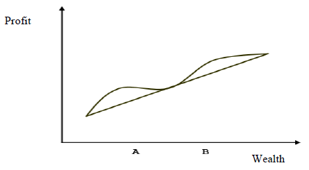
The presence of a paradox is worth noting: if rationality is assumed, why does the same individual buy both insurance and lottery tickets? This preference for lotteries and games of chance contradicts the theory of choice and profit postulates since its expected return is negative and reveals an attitude of passion for risk. Friedman and Savage (1948) 2 suggest that the profit curve takes different forms according to the income levels of individuals. The profit curve is composed of three segments3: it tends to be concave downward for low-income levels, concave upward for middle-income levels, and again concave downward for high-income levels (decreasing, increasing, and decreasing marginal profit, respectively).
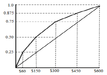
Figure 1 shows in A low-income levels where individuals present a downward concave profit curve and are risk-averse but like to participate in random games if such games can shift their wealth to PB and higher levels (where the profit curve is again downward concave). In the second category are individuals who prefer large-scale gambles. In the last segment are high-income individuals who prefer certainty relative to moderate and extreme risks. They prefer small winnings and reasonably safe games with the possibility of small losses. They are risk-averse individuals who seek a premium for taking moderate risks.4 This situation is depicted in Figure 2.
The theory of profit has been enriched in the last two decades with models considering the complexity of decision making. Several factors may shape individuals' preferences. For example, individuals may be concerned about the stability of their income levels and health; if their health has declined somewhat, they may place less value on their future income because of the impossibility of enjoying it fully. Likewise, instability in income levels alters consumption and savings patterns. Hence, in the face of a possible reduction in future income, many economic agents tend to save more as a preventive measure. This is precautionary saving. Attitudes such as these have been extensively analyzed by psychologists, economists, and actuaries, often in multidisciplinary studies. Analytically, the high-order derivatives of the profit function are examined.
Review of the literature
The application of copula models in various areas has grown considerably in recent years. They mainly analyze the dependence between random variables. Regarding tail dependence in financial series, Alqaralleh et al. (2019) study volatility in Stock Market prices at different time horizons and show that the skewness of the distribution can be modeled with a copula-EGARCH. In addition, Denkowska and Wanat (2020) propose a hybrid model for the dynamic analysis of interrelationships based on combining a copula-GARCH model and minimum spanning trees. As for research on dependence structures, Hamma et al. (2019) propose an optimal hedging strategy in oil reserves. The results show that the Gumbel copula is the best model. Li et al. (2019) analyze the dependence structure between the Chinese Stock Market and the RMB exchange rate showing significant structural breaks in the crisis period. Liao et al. (2019) use cluster copulas with GARCH models to measure the dependence between stock price and oil for G7 and BRICS countries; the empirical evidence shows a positive and significant dependence. Using copula-GARCH models, Chang et al. (2020) model China's emission rights and energy markets; the results show significant regional heterogeneity. Finally, Joseph et al. (2020) study the contagion in the global financial crisis and Eurozone crisis periods using bivariate vector error correction models estimated with GARCH (1,1), comparing Elliptic versus Archimedean copulas. The results show that the Clayton copula is the best fit for extreme dependence.
A couple of recent studies on dynamic models should be highlighted. Chen and Qu (2019) examine the leverage effect and dynamic correlation with copula between China's crude oil and precious metals. The result shows that the volatility of international crude oil and China's precious metals has a leverage effect. Furthermore, Li et al. (2020) propose a dynamic copula model combined with the ARIMA-GARCH model. The result shows that the proposed method can provide more accurate forecast error intervals.
In the case of Mexico, the literature on copulas is scarce. Venegas and Cruz (2010) and Durón et al. (2018) show empirical studies using more robust copulas models through the Archimedean type. García et al. (2017) incorporate Monte Carlo simulation in their study. Moreover, Olivares et al. (2017) propose Value-at-Risk models for the non-underestimation of market risk as an alternative to elliptic copula models applied to the Mexican housing sector, obtaining the best results for the t-Student.
Given the literature review, the current importance of the copula theory and the time series theory with its different applications to finance is evident. Therefore, this paper addresses this importance and proposes an adaptation of Merton's mean-variance portfolio.
Portfolio theory
The following equation expresses the investor's desired total return on their investment portfolio:
R: |
Investor's desired total return |
RR: |
Investor's actual desired return |
P: |
Premium for inflation risk |
PM: |
Market risk premium |
IP: |
Intrinsic risk premium |
The investor's desired real return is the income they obtain from their investment, i.e., they sacrifice their present consumption for the future, investing in the purchase of shares to increase their profit.
The investor's purchasing power loss due to inflation is compensated by a surcharge on the desired real return, equal to the inflation rate (π). The desired real rate of return (r) plus the premium for inflation risk determines the "risk-free rate" (TLR). This rate has the lowest risk of bank default; in Mexico, it is commonly available from Treasury Certificates (CETES).
The investor also wants a premium to compensate for the risks acquired by investing in assets other than risk-free assets, i.e., risky assets. This requires two types of premiums: a premium for market risk and a premium for the intrinsic risk of each company.
Market risk in the investor's profits or losses is due to changes in asset prices in the financial markets. Governmental policy decisions mainly cause this risk. Intrinsic risk is composed of commercial risk and financial risk. Commercial risk is caused by possible negative impacts that affect the efficiency of each company. Financial risk is caused by possible negative impacts on the yields of financial assets.
Merton mean-variance portfolio model
Based on the abovementioned characteristics of an investment, Merton (1972) revolutionized financial thinking. He contributed with a model for the construction of optimal investment portfolios by minimizing the risk of the portfolio subject to a given level of the portfolio's expected return. The solution to this problem is known as the mean-variance portfolio. Analyzing the construction of Merton's model, it turns out that the expected return of the portfolio is the weighted average of the expected returns of the assets that make up the portfolio:
|
Expected portfolio return p |
p : |
Asset portfolio |
wi: |
Weighting of the investment made in the i-th asset |
E(Ri) : |
Expected return on the i-th asset |
n: |
Number of assets |
The portfolio's risk is measured by its standard deviation with respect to its expected return. Luenberger (1998) states that the variance of portfolio returns is the weighted average of the covariances of all the pairs included in the portfolio, which is expressed as:
|
Variance of portfolio returns p |
wi wj: |
Weighting of investment in assets i and j |
σij: |
Variance between the returns of assets i and j if I = j, or covariance between the returns of assets i and j if I ≠ j. Or, in other words, expressed as a matrix, the following is obtained |
where:
W: |
vector of weights (proportions) of the assets |
WT: |
transposed from W |
Σ: |
variance-covariance matrix of the asset portfolio |
Analogously, the variance-covariance matrix can be decomposed using
Therefore, the estimation of the variance of the portfolio can be carried out using
It is worth mentioning that this decomposition of the variance and covariance matrix is the one that will be used to incorporate the copula and GARCH models. The copula models will be incorporated through the correlation parameters to form the correlation matrix, and the GARCH models will be incorporated through the volatility parameters to form the volatility matrix.
The expression of Equation (3) in its matrix form is equal to
Therefore, the standard deviation of the portfolio (risk) is
It is necessary to find the optimal weights (w1, w2, …,wn) that minimize the risk for each expected return to find the efficient frontier of the investment portfolios. Thus, the optimization problem posed by Merton is expressed as follows:
subject to:
The restriction is that the weights at least obtain a value of 0 to avoid allowing short sales in the model.
Copula theory
A copula function is a multivariate distribution function defined on the unit cube [0,1]n × [0,1], with uniformly distributed marginals. The mathematical basis of copula functions is established by Hoeffding (1940) and is specified by Sklar's Theorem (1959).
Sklar's theorem
Let it be an n-dimensional distribution function F with continuous marginal distributions F1,…,Fn; there exists a unique n-copula C: [0,1]n→[0,1], such that:
Then, the copula combines the marginals to form a multivariate distribution. This theorem provides a parameterization of the multivariate distribution and a copula construction diagram.
This theorem allows the choice of different marginals and a given dependence structure to be used in the construction of a multivariate distribution5. It differs from the traditional way of constructing multivariate distributions, where one has the restriction that the marginals are usually of the same type.
The copula functions to be used in this work are bivariate copulas—copulas composed of only two marginal distribution functions. It is important to note that the marginal distribution functions that will be used to construct the bivariate copula functions will be marginal distribution functions corresponding to the distributional structure that will be proposed through the copulas.
Although there are many copula functions, this paper will only focus on the copulas of the Elliptic family: the Gaussian copula and the t-Student copula.
The main characteristic of these copulas is that they are associated with random variables with a symmetrical multivariate distribution function. Therefore, the contour lines generated by this type of copulas have an elliptical shape.
Gaussian copula
The Gaussian copula is a generalization of a multivariate Gaussian distribution. For the bivariate case Φ denotes the (cumulative) Gaussian distribution, and Φρ,2 denotes the standard 2-dimensional Gaussian distribution with correlation matrix ρ.
The bivariate Gaussian copula with correlation matrix ρ is
As noted above, the marginal distribution functions used in this paper for the estimation of bivariate normal copulas correspond to the distributional structure of the copula, in this case Gaussian marginal.
T-Student copula
The t-Student copula is a generalization of a multivariate t-Student distribution. For the bivariate case, a 2-dimensional t-Student distribution T2,p,ν with ν degrees of freedom and a correlation matrix ρ is defined as
And its respective bivariate t-Student copula with correlation matrix ρ and ν degrees of freedom is
where Tν is the univariate t-Student distribution with ν degrees of freedom.
As indicated, the marginal distribution functions used for estimating the bivariate t-Student copulas correspond to the copula's distributional structure, in this case, t-Student marginals.
Estimation of copula parameters
The estimation of the parameters of the Elliptic copulas proposed in this work will be through the maximization of their log-likelihood function.
The log-likelihood function is defined as
where θ is the set of parameters of both the marginals and the copula.
The log-likelihood function is maximized, and the maximum likelihood estimator is obtained:
The estimated copula parameter (dependence parameter) will serve as the correlation parameter in the Merton portfolio. Thus, two correlation matrices will be generated, one with the parameters estimated via the Gaussian copula and the other with the parameters estimated via the t-Student copula.
GARCH model
Bollerslev (1986) extends the ARCH model, proposing the GARCH model6. The generalized autoregressive conditional heteroscedasticity (GARCH) model estimates that the conditional variance depends on two factors: the innovations of the squared residuals ε2 t-1, ε2 t-2, ε2 t-p, known as the ARCH effect, with their respective autoregressive coefficients; and the prior conditional variances σ2 t-1, σ2 t-2, σ2 t-p, known as the GARCH effect, with their respective autoregressive coefficients; an intercept term, γ0; and an error term, ut..
The GARCH model is expressed as
The GARCH model exemplifies a GARCH (p,q) model, where p and q determine the number of lags. It is necessary to mention that the sum of the autoregressive coefficients of the ARCH and GARCH effects must be less than or equal to 1, i.e., α0 + α1 +∙∙∙+ αp + β0 + β1 + ∙∙∙ + βq ≤ 1, so that the GARCH process is ensured to be stationary and ergodic.
This study uses the GARCH model with errors distributed in two different ways, specifically via the two distributional proposals proposed in the copula models: the Gaussian distribution and the t-Student distribution. Once the conditional variance of both models is obtained, its square root is extracted to obtain the adjusted standard deviation (volatility) that will be used in the configuration of the variance and covariance matrices that will be used in the configuration of the adjusted portfolios.
Analysis of results
This research considers the daily historical returns of the BMV Total Return Economic Activity Indices. The period covers ten years, from September 30, 2010, to September 30, 2020. Considering daily data, basic descriptive statistics of expected return, standard deviation, and Sharpe ratio [E(Ri) - TLR]/σi are estimated. After that, GARCH models are estimated to obtain the volatility estimation. Subsequently, correlation matrices are estimated, two of which incorporate the adjustment via copulas, to subsequently estimate the variance and covariance matrices that include the adjustment via copulas and GARCH models. Finally, three mean-variance investment portfolios are constructed: i) Merton mean-variance portfolio, ii) Merton portfolio with copula-GARCH-Gaussian fitting, and iii) Merton portfolio with copula-GARCH-t-Student fitting.
Figure 3 shows the behavior of the portfolio components (i.e., the selected BMV Total Return Economic Activity Indices), composed of both the prices and the returns of each of the indices under analysis. It should be noted that only five of the seven Total Return Economic Activity Indices were considered for the portfolio because the Sharpe ratios for the Mining, Agriculture, and Construction sectors were negative, i.e., expected returns were below the CETES reference rate.
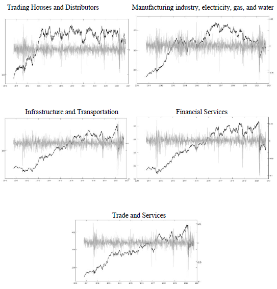
Source: created by the authors
Figure 3 Daily Returns and Prices of Total Return Economic Activity Indices
Table 1 shows the annualized results of the descriptive statistics, expected return and standard deviation, and the volatility estimation through the GARCH-Gaussian and GARCH-t-Student models corresponding to the indices analyzed.
Table 1 Descriptive Statistics and Volatility via GARCH Model of Total Return Economic Activity Indices
| Trading
Houses and Distributors |
Manufacturing
industry, electricity, gas, and water |
Infrastructure
and Transportation |
Financial
Services |
Trade and
Services |
|
| Expected
return |
0.052804 | 0.068908 | 0.081308 | 0.075215 | 0.087651 |
| Standard
deviation |
0.153779 | 0.151341 | 0.166487 | 0.187479 | 0.157322 |
| Gaussian
GARCH Volatility |
0.153161 | 0.151260 | 0.161210 | 0.173633 | 0.238656 |
| GARCH
t-Student Volatility |
0.148905 | 0.170043 | 0.158994 | 0.178541 | 0.154059 |
Source: created by the authors
Continuing with the analysis, the correlation, variance, and covariance matrices are obtained; first in a simple way, that is, via Pearson's correlation parameter and the Variance and Covariance estimator. Table 2 illustrates this.
Table 2 Correlation Matrix and Variance and Covariance Matrix of the Total Return Economic Activity Indices using the Merton model
| Panel A. Correlation Matrix | |||||
| Correlation | Trading
Houses and Distributors |
Manufacturing
industry, electricity, gas, and water |
Infrastructure
and transportation |
Financial
Services |
Trade and
Services |
| Trading Houses and Distributors | 1 | 0.76639583 | 0.61011699 | 0.61294556 | 0.82990711 |
| Manufacturing industry, electricity, gas, and water | 0.766395833 | 1 | 0.65878299 | 0.67045404 | 0.70313674 |
| Infrastructure and transportation | 0.610116992 | 0.65878299 | 1 | 0.66501256 | 0.76342621 |
| Financial Services | 0.612945562 | 0.67045404 | 0.66501256 | 1 | 0.66489603 |
| Trade and Services | 0.829907111 | 0.70313674 | 0.76342621 | 0.66489603 | 1 |
| Panel B. Variance and Covariance Matrix | |||||
| Variances
Covariances |
Trading
Houses and Distributors |
Manufacturing
industry, electricity, gas, and water |
Infrastructure
and transportation |
Financial
Services |
Trade and
Services |
| Trading Houses and Distributors | 0.023648008 | 0.01783641 | 0.01562038 | 0.01767147 | 0.02007786 |
| Manufacturing industry, electricity, gas, and water | 0.017836413 | 0.02290415 | 0.01659896 | 0.01902302 | 0.01674123 |
| Infrastructure and transportation | 0.015620383 | 0.01659896 | 0.02771804 | 0.020757 | 0.01999581 |
| Financial Services | 0.017671468 | 0.01902302 | 0.020757 | 0.03514851 | 0.01961091 |
| Trade and Services | 0.020077856 | 0.01674123 | 0.01999581 | 0.01961091 | 0.02475034 |
Source: created by the authors
Subsequently, the correlation matrices are obtained in an adjusted form; that is, the correlation matrices are generated via the copula methodology. They are created using the estimated parameters of the Elliptic copulas, the Gaussian copula, and the t-Student copula. It should be remembered that the adjustment of the marginals to be used in estimating the copulas is an adjustment of the proposed distributional assumption. Consequently, the marginals used in the Gaussian copula are Gaussian marginals, and those used in the t-Student copula are t-Student marginals.
The variance and covariance matrices are then generated. They include the GARCH models with Gaussian and t-Student innovations in addition to the estimated copulas. Table 3 contains the matrices generated with the Gaussian assumption, and Table 4 contains the matrices generated under the t-Student assumption.
Table 3 Correlation Matrix and Variance and Covariance Matrix adjusted via Gaussian copula and Gaussian GARCH of Total Return Economic Activity Indices Returns
| Panel A. Correlation Matrix (Gaussian Copula Parameters) | |||||
| Correlation | Trading
Houses and Distributors |
Manufacturing
industry, electricity, gas, and water |
Infrastructure
and transportation |
Financial
Services |
Trade and
Services |
| Trading Houses and Distributors | 1 | 0.76639583 | 0.61011699 | 0.61294556 | 0.82990711 |
| Manufacturing industry, electricity, gas, and water | 0.766395833 | 1 | 0.65878299 | 0.67045404 | 0.70313674 |
| Infrastructure and transportation | 0.610116993 | 0.65878299 | 1 | 0.66501256 | 0.76342621 |
| Financial Services | 0.612945562 | 0.67045404 | 0.66501256 | 1 | 0.66489602 |
| Trade and Services | 0.829907111 | 0.70313674 | 0.76342621 | 0.66489602 | 1 |
| Panel B. Variance and Covariance Matrix (Gaussian copula parameters and Volatility via Gaussian GARCH) | |||||
| Variances
Covariances |
Trading
Houses and Distributors |
Manufacturing
industry, electricity, gas, and water |
Infrastructure
and transportation |
Financial
Services |
Trade and
Services |
| Trading Houses and Distributors | 0.023458176 | 0.0177551 | 0.01506441 | 0.01630053 | 0.03033537 |
| Manufacturing industry, electricity, gas, and water | 0.017755103 | 0.02287947 | 0.01606413 | 0.01760859 | 0.02538256 |
| Infrastructure and transportation | 0.015064414 | 0.01606413 | 0.02598867 | 0.01861463 | 0.02937188 |
| Financial Services | 0.016300528 | 0.01760859 | 0.01861463 | 0.03014847 | 0.02755238 |
| Trade and Services | 0.030335373 | 0.02538256 | 0.02937188 | 0.02755238 | 0.05695678 |
Source: created by the authors
Table 4 Correlation Matrix and Variance and Covariance Matrix adjusted via t-Student and GARCH t-Student copula of Total Return Economic Activity Indices Returns
| Panel A. Correlation Matrix (t-Student Copula Parameters) | |||||
| Correlation | Trading
Houses and Distributors |
Manufacturing
industry, electricity, gas, and water |
Infrastructure
and transportation |
Financial
Services |
Trade and
Services |
| Trading Houses and Distributors | 1 | 0.76648243 | 0.6103059 | 0.61306397 | 0.83022615 |
| Manufacturing industry, electricity, gas, and water | 0.766482429 | 1 | 0.65903221 | 0.67053539 | 0.70339153 |
| Infrastructure and transportation | 0.610305904 | 0.65903221 | 1 | 0.6649836 | 0.76356016 |
| Financial Services | 0.613063971 | 0.67053539 | 0.6649836 | 1 | 0.66496015 |
| Trade and Services | 0.830226155 | 0.70339153 | 0.76356016 | 0.66496015 | 1 |
| Panel B. Variance and Covariance Matrix (t-Student copula parameters and Volatility via GARCH t-Student) | |||||
| Variances
Covariances |
Trading
Houses and Distributors |
Manufacturing
industry, electricity, gas, and water |
Infrastructure
and transportation |
Financial
Services |
Trade and
Services |
| Trading Houses and Distributors | 0.022172755 | 0.0194075 | 0.01444898 | 0.01629868 | 0.01904552 |
| Manufacturing industry, electricity, gas, and water | 0.019407498 | 0.02891446 | 0.01781738 | 0.0203571 | 0.01842643 |
| Infrastructure and transportation | 0.014448976 | 0.01781738 | 0.02527897 | 0.01887676 | 0.01870293 |
| Financial Services | 0.016298679 | 0.0203571 | 0.01887676 | 0.03187671 | 0.01829022 |
| Trade and Services | 0.019045521 | 0.01842643 | 0.01870293 | 0.01829022 | 0.02373413 |
Source: created by the authors
Once the variance and covariance matrices for each of the proposed cases are available, the implementation of the diversification of the portfolios is continued. Table 5 shows the weights of the diversified portfolios composed of the BMV Total Return Economic Activity Indices. The weights considering the Merton model and those considering the models adjusted via GARCH and copula models are shown. It is worth remembering that the estimated diversification was carried out with the objective function of minimizing the variance of the portfolio, considering the restrictions of the Merton model.
Table 5 Mean-variance portfolio of BMV Total Return Economic Activity Indices
| Indices | Weight
Merton Model |
Weight
Gaussian-GARCH Copula |
Weight
GARCH t-Student copula |
| Trading Houses and Distributors | 0.30337156 | 0.3312723 | 0.53888521 |
| Manufacturing industry, electricity, gas, and water | 0.35845296 | 0.28824643 | 0 |
| Infrastructure and transportation | 0.2353614 | 0.27729635 | 0.36033337 |
| Financial Services | 0.01264034 | 0.10318492 | 0.10078141 |
| Trade and Services | 0.09017374 | 0 | 0 |
| SUM | 1 | 1 | 1 |
Source: created by the authors
It is important to note in Table 5 that the algorithm for the GARCH-Gaussian copula rules out investment in the Trade and Services index, while the GARCH-t-Student copula, being more restrictive, in addition to ruling out investment in the Trade and Services index, also does so for Manufacturing Industry and Electricity, Gas and Water. Likewise, it is observed that the Merton model does not rule out investing in any of the indices that make up the portfolio.
Table 6 shows the risk-return relationship of the mean-variance portfolio obtained through the diversification of the three proposed portfolios.
Table 6 Risk and Return in the mean-variance portfolio of BMV Total Return Economic Activity Indices
| Standard deviation | Expected return | |
| Mean-variance portfolio | 0.13884507 | 0.06871079 |
| Gaussian GARCH mean-variance portfolio and Gaussian copula | 0.13692394 | 0.06766236 |
| Mean-variance GARCH t-Student and t-Student copula portfolios | 0.13710442 | 0.06533333 |
Source: created by the authors
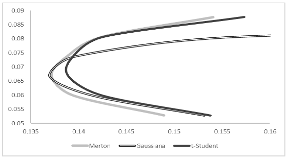
The information in Table 6 can be seen in Figure 4, which shows the three efficient frontiers generated through the proposed portfolios. The difference between these three frontiers is visible, highlighting the difference in the estimated values of the mean-variance portfolio (vertex of the parabola) where the minimum risk is found. It can be concluded that the Merton model of investment portfolios applied to the BMV Total Return Economic Activity Indices underestimates return and risk, as does the GARCH-Gaussian copula-adjusted portfolio because it is very similar in its behavior, unlike the GARCH-t-Student copula-adjusted portfolio, which clearly does not underestimate risk. The main implication of not underestimating risk in the efficient frontier is that the t-Student distribution better captures the fluctuations the portfolio may have, i.e., it is closer to reality. Therefore, when there is an underestimation, the expected results can be very different from the real ones, especially in times of crisis.
Conclusions
This research conducted a diversification analysis. Three investment portfolios comprising the BMV Total Return Economic Activity Indices were considered. A Merton mean-variance portfolio and two portfolios adjusted via copula and GARCH models with an Elliptic support were generated. The efficient frontiers obtained from each of the portfolios were contrasted, and it was concluded that the Merton mean-variance portfolio model and the copula-GARCH-Gaussian model applied to the BMV Total Return Economic Activity Indices underestimate return and risk, while the copula-t-Student portfolio does not. By breaking the constant volatility assumption, the best results in terms of not underestimating risk are observed in the GARCH-t-Student copula since this copula is leptokurtic, which contributes to effectively capturing the volatility clusters in the returns of the BMV Total Return Economic Activity Indices. This is reflected in the comparison of efficient frontiers in the determined models. For future research, more robust portfolios can be constructed through Archimedean copulas.
REFERENCES
Alqaralleh, H., Awadallah, D., y Al-Ma’aitah, N. (2019). Conectividad financiera asimétrica dinámica bajo dependencia de cola y variación de tiempo procesada: evidencia seleccionada de los mercados de valores emergentes de MENA. Borsa Istanbul Review, vol. 19, num. 4, pp. 323-330. https://doi.org/10.1016/j.bir.2019.06.001 [ Links ]
Bardsley, N., Cubitt, R., Loomes, G., Moffatt, P., Starmer, C., and Sugden, R. (2009). Assessing Experimental Economics. Princeton: Princeton University Press. https://doi.org/10.1515/9781400831432 [ Links ]
BMV (01 de febrero de 2021). Índices de actividad económica. Recuperado de: https://www.bmv.com.mx/es/indices/actividadeconomica/ [ Links ]
Bollerslev, T. (1986). A conditionally heteroskedastic time series. Model for speculative prices and rates of return. The Review of Economics and Statistic, 69(3). pp. 542-547. https://doi.org/10.2307/1925546 [ Links ]
Brink, A.G., Hobson, J. y Stevens, D.E. (2012). The Effect of Financial Incentives on Excessive Risk-Taking Behavior: An Experimental Examination Incorporating Earnings management and Individual Factors. Working Paper, Virginia Commonwealth University. https://doi.org/10.2139/ssrn.2046415 [ Links ]
Chang, K., Zhang, C., y Wang, H. (2020). Estructuras de dependencia asímétrica entre derechos de emission y mercados de energía: nueva evidencia de los pilotos del esquema de comercio de emisiones de China. Ciencias Ambientales e Investigación de la Contaminación, vol. 27, num. 17, pp. 21140-21158. https://doi.org/10.4272/978-84-9745-224-3.ch6 [ Links ]
Chen, Y., y Qu, F. (2019). Leverage effect and dynamics correlation between international crude oil and China’s precious metals, Physica A: Statistical Mechanics and its Applicationss, vol. 534. https://doi.org/10.1016/j.physa.2019.122319 [ Links ]
Cherubini, U., Luciano, E. y Vecchiato, W. (2004). Copula methods in finance. John Wiley & Sons. England. https://doi.org/10.1002/9781118673331 [ Links ]
Copeland, T., Weston, J.F. y Shastri, K. (2005). Financial Theory and Corporate Policy. Pearson Addsion-Wesley. [ Links ]
Cox, J.C. y Sadiraj, V. (2006), Small-and large-stakes risk aversion: Implications of concavity calibration for decision theory. Games and Economic Behavior, vol. 56, num.1, pp. 45-60. https://doi.org/10.1016/j.geb.2005.08.001 [ Links ]
Denkowska, A., y Wanat, S. (2020). A Tail Dependence-Based MST and Their Topological Indicators in Modeling Systemic Risk in the European Insurance Sector. Risks, vol. 8, num. 2. https://doi.org/10.3390/risks8020039 [ Links ]
Direr, A. (2012). Can Expected Utility Explain MultiplePrize Lotteries?, Working Paper, Université d’Orleans. https://doi.org/10.1257/00028280260136426 [ Links ]
Durón, N., Cruz, S., y Venegas, F. (2018). Determinación del capital económico requerido para cubrir el riesgo de desastres naturales en Veracruz, México: un enfoque de cópulas arquimedianas, EconoQuantum, vol. 15, num. 1, pp. 7-29. https://doi.org/10.18381/eq.v15i1.7110 [ Links ]
Einsehauer, J.G. (2005). How Prevalentare the Friedman-Savage Utility Functions?, Briefing Notes in Economics. Issue 66. [ Links ]
Friedman, M., y Savage, L. (1948). The Utility Analysis of Choices Involving Risk. Journal of Political Economy, vol. 56, num. 4, pp. 279-303. https://doi.org/10.1086/256692 [ Links ]
García, R. S., López, F., y Cruz, S. (2017).CDS pricing using a Copula-Monte Carlo Approach, Revista de Investigación en Ciencias Contables y Administrativas, vol. 3, num. 1, pp. 111-133. [ Links ]
Hamilton, J. D. (1994). Time Series Analysis. Princeton University Press. Estados Unidos. https://doi.org/10.1017/s0266466600009440 [ Links ]
Hamma, W., Salhi, B., Ghorbel, A., jarboul, A. (2019). Estructuras de dependencia condicional entre los precios del petróleo y los mercados bursátiles internacionales: implicación para la gestión de la cartera y la eficacia de la cobertura. Revista Internacional de Gestión del Sector Energético, vol. 14, num. 2, pp. 439-467. https://doi.org/10.32719/25506641.2020.8.5 [ Links ]
Harrison, G. W. (1994). Expected Utility Theory and the Experimentalists, Empirical Economics, vol. 19, num. 2, pp. 223-54. https://doi.org/10.1007/978-3-642-51179-0_4 [ Links ]
Heukelom, F. (2009). Kahneman y Tversky and the Origin of Behavioral Economics. Ph. Thesis, Amsterdam School of Economics. https://doi.org/10.2139/ssrn.956887 [ Links ]
Hoeffding, W. (1940). Masstabinvariante Korrelationstheorie, Schriften des Mathematischen Instituts und des Instituts für Angewandte Mathematik der Universität Berlin, vol. 5, pp. 179-223. [ Links ]
Joseph, N., Vo, T., Mobarek, A., y Mollah, S. (2020). Volatility and asymmetric dependence in Central and East European stock markets. Review of Quantitative Finance and Accounting, 55(1), 1241-1303. https://doi. org/10.1007/s11156-020-00874-0 [ Links ]
Li, L., Miao, S., Tu, Q., Duan, S., Li, Y., y Han, J. (2020). Modelado de dependencia dinámica de la incertidumbre de la energía eólica considerando el efecto heteroscedástico. Revista Internacional de Energía Eléctrica y Sistemas de Energía, vol. 11, num. 6. https://doi.org/10.31428/10317/3118 [ Links ]
Li, R., Hu, Z., Li, S., y Yu, K. (2019). Estructuras de dependencia dinámica entre los rendimientos del mercado de valores chino y los tipos de cambio del RMB. Mercados emergentes Finanzas y comercio, vol. 55, num. 15, pp. 3553-3574. https://doi.org/10.18046 [ Links ]
Liao, R., Boonyakunakorn, P., Liu, J., y Sriboonchitta, S. (2019). Modelado de estructuras de dependencia de los precios del petróleo crudo y los mercados de valores de los países desarrollados y en desarrollo: un enfoque de copula C-vine. Revista de Física: serie de conferencias, vol. 1324, num. 1. https://doi.org/10.1787 [ Links ]
Luce, R.D. (1999). Utility Gains and Losses: Measurement-Theoretical and Experimental Approaches. New York: Laurence Erlbaum Associates. https://doi.org/10.4324/9781410602831 [ Links ]
Luenberger, D.G. (1998). Investment Science. Oxford University Press. [ Links ]
Merton, R. C. (1972). An Analytic Derivation of the Efficient Portfolio Frontier. The Journal of Financial and Quantitative Analysis, vol. 7, num. 4. https://doi.org/10.2307/2329621 [ Links ]
Nelsen, R. B. (2006). An introduction to copulas. Springer. Estados Unidos. [ Links ]
Olivares, H. A., Bucio, C., Agudelo, G. A., Franco, L. C., y Franco, L. E. (2017). Valor en Riesgo: Un análisis del modelo de cópulas elípticas para el sector de vivienda en México, Espacios, vol. 38, num. 31, pp. 27-52. [ Links ]
Sánchez, A. y Reyes, O. (2005). Regularidades probabilísticas de las series financieras y la familia de modelos GARCH. Ciencia Ergo Sum, vol. 13, num. 2, pp. 149-156. [ Links ]
Sklar, A. (1959). Fonctions de Répartition à n Dimensions et Leurs Marges. Publications de l’Institut Statistique de l’Université de Paris, vol. 8, pp. 229-231. [ Links ]
Venegas Martínez, Francisco y Salvador Cruz, Aké (2010). Valuación de bonos corporativos mediante cópulas arquimedeanas y marginales de valores extremos. En Ortiz Arango, Francisco (Editor). Avances recientes en valuación de activos y administración de riesgos, Volumen 1, Universidad Panamericana: México. pp. 69-102. https://doi.org/10.22201/fca.24488410e.2007.621 [ Links ]
1A good summary on experimental and empirical studies on utility and the behavior of economic agents can be found in Copeland et al. (2005); see also Harrison (1994), Luce (1999) and Cox and Sadiraj (2006), Bardsley et al. (2009) and Brink, Hobson, and Stevens (2012).
2Milton Friedman received the Nobel Prize in Economics in 1976 "for his achievements in the fields of consumption analysis, monetary history and theory, and for his demonstration of the complexity of stabilization policy."
4Since its inception, the Friedman-Savage paradox has been the subject of much debate. Recent examples of these debates can be found in Einsehauer (2005), Heukelom (2009), and Direr (2012).
5For further information on Copula Theory see Nelsen (2006) and Cherubini et al. (2004).
6It should be noted that only one methodology of the GARCH family—the traditional GARCH model—will be specified in this study. For a better understanding of these models and a description of other models belonging to the GARCH family, see Hamilton (1994), and Sanchez and Reyes (2005).
Received: June 24, 2020; Accepted: March 03, 2021; Published: March 08, 2021
 Este es un artículo publicado en acceso abierto bajo una licencia Creative Commons
