Introduction

If an organization has a choice between oil and gas to produce electricity, it will use oil when it is less expensive than gas and gas when it is less expensive than oil. That is, the organization uses either energy source to minimize production costs. Substitution of that source generates price competition between oil and gas for supply and demand. The price of gas is usually lower than the price of oil, but there are periods when the relation is inverse.

^{Hartley et al. (2008)} analyze the relation between natural gas and crude oil prices, concluding that the relation between gas and oil prices is indirect, technology is important for the long-term relation between prices, and short-term deviations are influenced by inventories, weather, and seasonal factors. ^{Venegas Martinez (2008)} presents the valuation of options with Lévy processes.

^{Moutinho et al. (2011)} analyze the short-run dynamics between commodity prices and electricity prices in Spain from 2002 to 2005 and the long-run relation between the stochastic trends of fuel, gas, coal, and Brent prices. They conclude that in the long run, the relation of gas and Brent prices is correlated and that the price of gas explains the price of electricity.

^{Dahl et al. (2012)} indicate that gas prices in the UK spot market follow a similar pattern as the international oil price, the gas spot market is more liquid, an increasing proportion of gas is used to generate electricity, competing with coal and nuclear, and an increasing level of natural gas is imported. They find that the stochastic trend of Brent is less predominant than that of National Balancing Point gas.

^{Murphy and Oliveira (2013)} examine the pricing of option contracts on the strategic petroleum reserve and consider how it is likely to be used by the government or refineries. The analysis shows that strategic petroleum reserve management produces social welfare.

^{Atil et al. (2014)} analyze the translation of oil prices into gas and gasoline prices, concluding that oil prices influence gas and gasoline prices. ^{Joëts (2014)} analyzes price translations in European energy futures markets (oil, gas, coal, and electricity) with maturities of 1, 10, 20, and 30 months in periods of normal and extreme volatility, showing that the increases in energy prices are more marked with extreme volatility, while they are almost nonexistent with normal volatility. In other words, energy markets behave like financial assets, and portfolio diversification is more profitable in the long run.

^{González Pedraza et al. (2014)} analyze the behavior of energy price risk, where the exposure to energy markets is a portfolio of oil, gas, coal, and electricity that models energy returns with generalized hyperbolic conditional distributions with daily energy futures data from August 2005 to March 2012. The analysis shows the importance of leptokurtosis and skewness in the distribution of energy risk factors, concluding that risk measures for energy portfolios with standard methods and in models with exponential extreme decay underestimate risk, particularly for short positions and short-termism.

^{Stern (2014)} indicates that international gas prices reflect the market fundamentals of the 1970s and 1990s, when gas replaced oil and oil derivatives, and that gas and oil are energy sources competing with other energy products, such as coal.

^{Kilian (2015)} indicates that oil price shocks have been recurring since the 1970s. The author shows the evolution of the U.S. oil price from a historical perspective and compares it with the price of coal and gas, concluding that positive oil shocks are associated with recessions in importing countries and that an increase in the oil price is a sign of scarcity and a precondition for the development and adoption of alternative energy technologies.

^{Schöne (2015)} indicates that modeling the cash flows of an investment project deserves attention in the valuation of real options on commodities where an empirical study reveals that prices are not stationary and have returns that do not exhibit a Gaussian distribution. The results suggest that the choice of the stochastic process has significant implications for valuation and optimal investments.

^{Gatfaoui (2015)} states that the prices of energy products are based on factors such as development and delivery costs, i.e., supply. The balance between demand and supply determines the prices of energy products that depend on seasonal and periodic weather effects (temperature, rainfall, or humidity). Supply and demand depend on production costs. Electricity generation is the result of transforming fossil fuels (oil, gas, and coal), so there is a correlation among the prices of electricity, oil, and gas: consumers use gas compared to oil products. Gas consumption depends on the price differential with oil. Gas consumption generates efficiency gains in the transportation industry, while the heavy truck sector has tax incentives to substitute oil with gas. The electricity sector chooses oil or gas as an energy source to produce electricity, managing substitution opportunities. The substitution process requires investment (equipment or technology), which explains the limitations of the opportunities for substituting oil or oil products with gas after 2005 and that result from the investments in infrastructure necessary to enable substitution. Substitution between oil and gas establishes implicit gas prices and price competition between the two energy sources. The ability of consumers to switch from oil to gas or from gas to oil contributes to the stabilization process. Organizations arbitrage the oil and gas price differential to accommodate the efficiency differences between oil and gas as energy sources. In New York and New England, approximately 30% of electricity generation is a result of energy switching, and given the shortage of gas in cold periods, increases in energy consumption are generated and gas is the main energy source. Hence, power plants use oil to produce electricity and satisfy energy switching by compensating for the shortfall in gas supply.

^{Shahmoradi and Swishchuk (2016)} indicate that oil price returns exhibit a distribution with heavy extremes and skewness (leptokurtosis and skewness). They then use the inverse Gaussian process, the diffusion process with jumps, and the gamma variance process as three Lévy processes with extremes with a higher frequency than the Gaussian distribution. They use the fast fractional Fourier transform to calibrate the parameters with data from European options on oil futures and conclude that these three Lévy processes perform best out of the sample of at-the-money options. ^{Václavík and Klimešová (2016)} analyze the valuation of gas-exchange options, which are a set of put options on a spread between the prices of various energy commodities, and indicate that the valuation model is important.

^{Arrigoni et al. (2019)} state that the Canadian government introduced a carbon tax to reduce greenhouse gas emissions. They define a carbon pricing approach and carbon price as the tax needed to motivate electricity producers to switch from coal to natural gas. They model prices under three stochastic procedures: inverse Gaussian, Gaussian, and Heston, concluding that the inverse Gaussian process outperforms the Gaussian and Heston processes because it considers the nature of energy prices.

^{Hilliard and Hilliard (2019)} develop a diffusion model with jumps for valuation and hedging with margined options on Brent futures. Model parameter estimation and out-of-sample pricing errors are calculated using data on Brent crude oil contracts. They conclude that an option on an underlying equity is effectively hedged by a portfolio with two margined options and the underlying.¹

^{Fang and Chag (2020)} use the fast fractional Fourier transform to analyze the efficiency of option pricing with the Lévy process. The results indicate that compared with the Gaussian model, the calibration errors for the Lévy process are smaller. They conclude that the parameter estimation makes the price valuation more accurate, reducing the risk of poor option valuation.

This paper is organized as follows: in section 2, the procedure for structuring the portfolio with the risk-free bond and the European put option on the relation between gas and oil prices is explained, and the definition of the α-stable distributions and the proposed model for the valuation of the European αstable put options are presented. In section 3, the analysis of the distribution of returns is carried out with the estimation of the descriptive statistics and the α-stable parameters; the Kolmogorov and Smirnov and Anderson and Darling goodness-of-fit tests are performed to justify the relevance of the α-stable distribution; and the fits of the Gaussian, α-stable, and t-Student distributions with the absolute frequencies of the returns are presented. In section 4, the European put options are valued, and a sensitivity analysis is performed. Finally, section 5 presents the conclusions and the bibliographical references.

Structured product

This section presents the theoretical framework and explains the procedure for the valuation of the European option to swap oil for gas.

Analysis of the distribution of returns

With the data under consideration, the relation between the gas and oil prices with the data sample is calculated.

Distribution fits

The fits of the a-stable, t-Student and Gaussian distributions to the absolute frequencies of the returns are presented in Figure 1.

Source: created by the authors with data from Banxico and EIA

Figure 1 Return fits 

The results in Tables 3 and 4 indicate that α-stable or t-Student³ distributions are more efficient than Gaussian or generalized extreme value distributions for modeling the empirical behavior of returns. Therefore, α-stable distributions are relevant for modeling returns and managing market risks (price risk).

Figure 1 presents the fits to the distributions, and the fits indicate that the estimation of the α-stable distribution is relevant for the valuation of the European put option on the relation of gas and oil prices.

Valuation of the european put option

Estimating α-stable parameters for risk-neutral density and goodness-of-fit tests justifies the valuation of European put options on the relation of gas and oil prices to exchange oil for gas. Then, with the data of July 19, 2019, the valuations of European put options are performed with the following initial factors: M₀ = 0.2284 , γ = 0.7148, i = 0.0822, r = 0.0188 and S =1 with hedging business periods from July 22, 2019, to March 13, 2020.

Options are a contingent right dependent on the underlying price at the maturity date, so the valuation of European options is performed with the Gaussian and α-stable models. The performance of the underlying during the hedging period is presented in Figure 2.

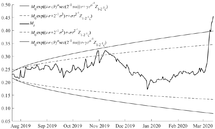
Source: created by the authors with data from Banxico, Federal Reserve, and EIA

Figure 2 Oil and gas relation performance 

Figure 2 presents the performance of the underlying, which indicates that on March 11, 12, and 13, 2020, the underlying breaches the upper bound of the α-stable confidence interval of 99% because the price of oil declined from 35.75 to 25.93. If the underlying price is greater than or equal to the settlement price (M_T ≥ S) then the structured product (portfolio) has bounded profits because the long position of the bond and the obligations for the settlement payment of the short option position are zero; therefore, the portfolio's value is Πt=S+p(t,Mt)exp⁡(iT). Otherwise (M_T < S), the structured product has smaller gains because the settlement payment obligations are equal to the energy cost savings paid by the long bond position; so, the portfolio value is Πt=pt,Mtexp⁡iT+MT. Therefore, the increase in the underlying price increases the portfolio's earnings. The valuation of European put options using Equations (7)-(9) is presented in Figure 3.

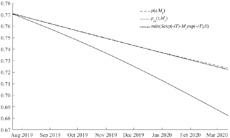
Source: created by the authors with data from Banxico, Federal Reserve, and EIA

Figure 3 Valuation of European put options 

Figure 3 presents the valuation of Gaussian, a-stable, and lower bound options for the hedging business period and indicates that Gaussian options overestimate price risk, and α-stable options minimize arbitrage opportunities because the price of European α-stable put options written on the relation between gas and oil prices is the lower bound of Equation (9), i.e., pαt,Mt=máx(Sexp⁡-iτ-Mtexp⁡-rτ,0). The valuation of European put options with expiration dates on Fridays in the middle of each month is presented in Table 5.

Table 5 presents the valuation of the Gaussian, α-stable, lower bound, intrinsic value, and portfolio utility options, and indicates that the value of the options decreases as the hedge period increases, the underlying prices are less than the settlement price (S =1) in the short term, the proposed hedge is efficient in the short term, the savings (intrinsic value) from the energy cost decrease in inverse proportion with the increase in the underlying price, and the portfolio profits increase in direct proportion with the increase in the underlying price. The structured product has a minimum guaranteed principal equivalent to the valuation of put option pαt,Mtexp⁡iT reversed at the risk-free interest rate during the term and a maximum gain equal to the face value of the bond and put option S+pa(t,Mt)exp⁡(iT) on the maturity date. The savings performance is presented in Figure 4.

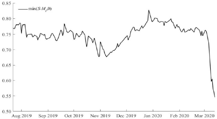
Source: created by the authors with data from Banxico, Federal Reserve, and EIA

Figure 4 . Intrinsic value 

Figure 4 presents the energy cost savings and indicates that they are equivalent to the payoff and

decrease in inverse proportion to the increase in the underlying price. The proposed hedge of the structured product is efficient because when the underlying price exceeds the upper limit of the confidence interval, the portfolio allows the trading of oil for gas and obtaining a profit equivalent to the product of the oil price and the put option on the maturity PTpα(t,Mt)exp⁡(iT) considering the energy cost of gas. The value of the structured product is presented in Figure 5.

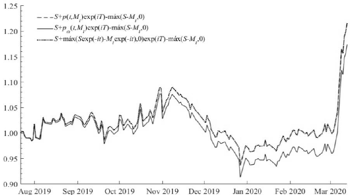
Source: created by the authors with data from Banxico, Federal Reserve, and EIA

Figure 5 Value of the structured product 

Figure 5 presents the value of the structured product at maturity date and indicates that the portfolio's value is pαt,Mtexp⁡iT+Mt because the underlying price is lower than the settlement price (M_T < S) and the portfolio's value increases in direct proportion to the increase in the underlying price. The hedge is efficient because it allows the trading of oil for gas and earning a profit equal to the product of the oil price and the put option PTpα(t,Mt)exp⁡(iT) on the maturity date— assuming that the premium for the exchange rate risk is invested at the domestic risk-free interest rate during the hedge period— then PTpαt,Mtexp⁡iT+Mt-Gt considers the energy cost of trading oil for gas. Then the proposed hedge is efficient when the underlying price is greater than or equal to the settlement price because the organization continues to produce electricity with oil when the price of oil is lower than the price of gas.

Sensitivity analysis

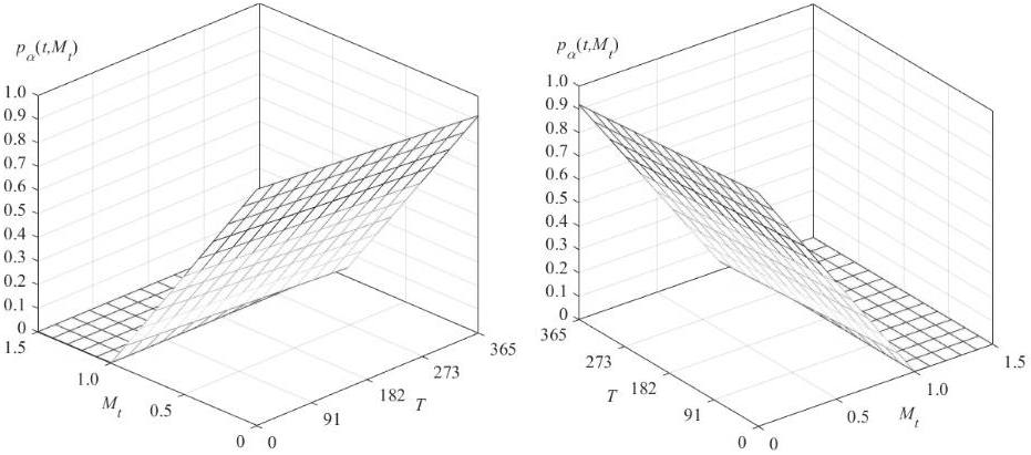
The sensitivity analysis evaluates the efficiency of the structured product for the organization's energy hedging, or equivalently, the ability to exchange oil for gas in the short term. The valuation of options where the underlying price varies in the interval 0 ≤ M_t ≤ 1.5 and with hedging periods in the interval 1 ≤ T ≤ 365 days is presented in Figure 6.

Source: created by the authors with data from Banxico, Federal Reserve, and EIA

Figure 6 Sensitivity analysis with respect to period and price 

Figure 6 presents the valuation of the options as a function of the hedge period and underlying price and confirms that the value of the options decreases as the hedge period increases; it decreases as the underlying price on the trade date increases to equal the settlement price where the options have zero value. The strategy is effective, and the valuation of the α-stable options adequately quantifies the price risk because when the options are traded in-the-money (M_t < S), then the value of the structured product on the expiration date allows oil to be traded for gas and the profit is PTpα(t,Mt)exp⁡(iT), or allows the use of oil and the profit is PTpαt,Mtexp⁡iT=PT(S-MT). When the options are traded or out-of-the-money (M_t ≥ S) and the options are in-the-money at the maturity date, then the portfolio's value is M_T, the option allows oil to be traded for gas, and the profit is PTMT-GT=0 i.e., null, but considering the energy cost of gas for production. When the options are out of the money, then the portfolio value is S and the profit is PTS-PT=0. Therefore, when the options are in-the-money on the settlement date, the organization minimizes the energy cost with the hedge generated from the structured product by trading oil for gas, generating savings maximized as the underlying price approaches zero and minimized as the underlying price approaches the settlement price. When the options are out-of-the-money (M_T < S), the organization continues to generate power with oil because the price of oil is lower than the price of gas. The probability that the European α-stable put options are in-the-money as a function of the underlying price and the term is presented in Figure 7.

Source: created by the authors with data from Banxico, Federal Reserve, and EIA

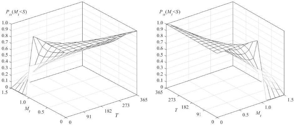
Figure 7 Probability of exercise with respect to period and price 

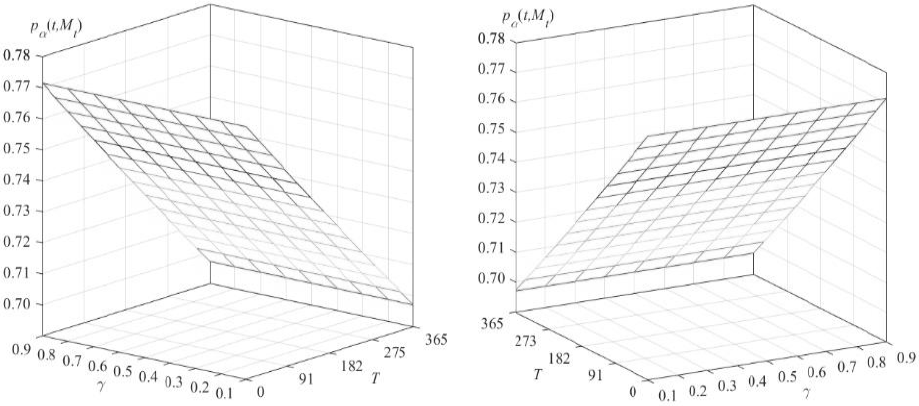
Figure 7 presents the probabilities of options being in-the-money as a function of the hedge period and the underlying price and indicates that the probabilities of trading oil for gas decrease as the underlying price increases and increase as the hedge period increases; so the probabilities of options being out-of-the-money are decreasing with respect to the underlying price. Therefore, the probabilities of the options being out-of-the-money are decreasing with respect to the underlying price and increasing with respect to the hedging period. The valuation of options with varying volatility in interval 0.1 ≤ γ ≤ 0.9 and with hedging periods in interval 1 ≤ T ≤ 365 days is presented in Figure 8.

Source: created by the authors with data from Banxico, Federal Reserve, and EIA

Figure 8 Sensitivity analysis with respect to period and volatility 

Figure 8 presents the valuation of options as a function of the hedge period and the scaling parameter. It confirms that the value of the options decreases as the hedging period increases and is constant with the change in volatility because the lower bound on the value of the European put options is máx(Sexp-iτ-Mtexp⁡-rτ,0). The valuation of the options varying the risk-free interest rate in the interval 0.01 ≤ i ≤ 0.15 and with hedging periods in the interval 1 ≤ T ≤ 365 days is presented in Figure 9.

Source: created by the authors with data from Banxico, Federal Reserve, and EIA

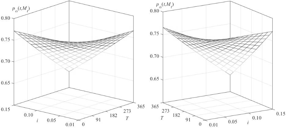
Figure 9 Sensitivity analysis with respect to period and rate 

Figure 9 presents the valuation of the options as a function of the hedge period and interest rate and indicates that the value of the options is a convex function that decreases as the hedge period or interest rate increase. The valuation of the options varying the settlement price in the interval 0.1 ≤ S ≤ 1 and with hedging periods in the interval 1 ≤ T ≤ 365 days is presented in Figure 10.

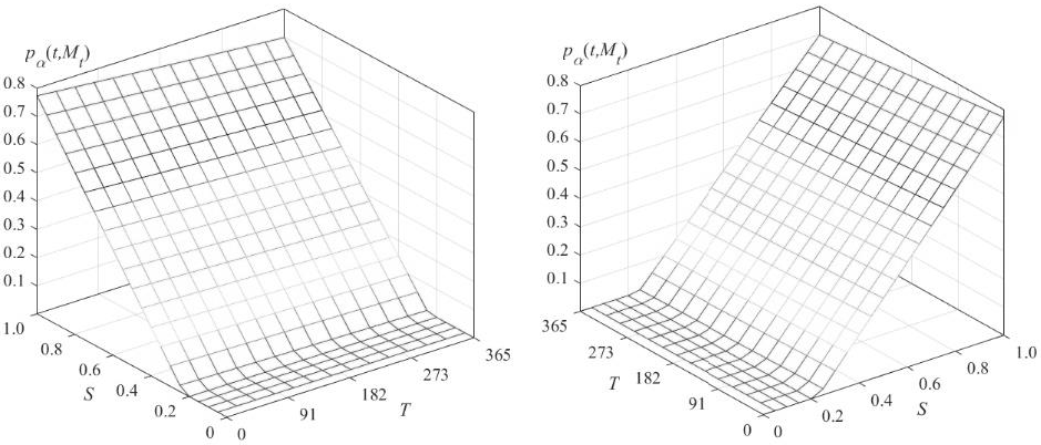
Source: created by the authors with data from Banxico, Federal Reserve, and EIA

Figure 10 Sensitivity analysis with respect to period and settlement price 

Figure 10 presents the valuation of the options as a function of the hedging period and the settlement price presented, and indicates that the value of the options is a convex function that decreases as the hedging period increases, and increases as the interest rate increases.

The sensitivity analysis indicates that the savings and energy costs of switching from oil to gas or continuing to use oil to produce electricity, respectively, are maximum when the underlying price approaches zero and minimum when the underlying price approaches the settlement price. The organization's strategy using the structured product is financially efficient, even when the settlement price is less than unity because the value of the portfolio minus the energy cost of production is:

PTS+pαt,Mtexp⁡iT-máx(S-MT)-mínGT,PT.

Then, if the price of gas is lower than the price of oil, the organization's profit is PTpαt,Mtexp⁡(MT), and if the price of oil is lower than the price of gas, hedging is efficient when S+pαt,Mtexp⁡(iT))≥1.

The above results exhibit that α-stable options are statistically more efficient than Gaussian options in quantifying market risk, specifically price risk. The prices and profits of α-stable options are lower than those of Gaussian options, and the use of gas is less costly than the use of oil to generate electric power during the study period.

Conclusions

The structured product is analyzed as a diversified portfolio with a long position in a domestic risk-free bond and a short position in a European put option issued on the relation between the price of gas and the price of oil with a risk and return profile that is difficult to replicate with doubtful or capital market products and provides access to a synthetic underlying.

Investors are generally unaware of the characteristics or valuation method, and their information is focused on the payout diagrams and not on the probability of the contingent payout of the portfolio. On the other hand, the issuers of the structured product hedge implicit risks by using derivative products, in this case, a European put option.

The structure provides policies to minimize production costs to increase the competitiveness of electricity-producing organizations. Changes in the price of oil generate changes in the energy costs of electricity production that have economic consequences because energy costs are reflected in profits and consumption.

The opportunity assumption to substitute oil with gas persists in the face of changes in oil and gas prices, and the creation of hedges to minimize production costs generates savings that promote competition. Parameter estimation and fit to the α-stable distribution confirm the ability to substitute one energy source with an alternative source with a lower price and the innovation with a guaranteed capitalstructured product with the statistical justification of a stochastic α-stable process of the underlying return because the descriptive statistics indicate that the underlying returns are leptokurtic and skewed. The Gaussian assumption of the analyzed returns is rejected with goodness-of-fit tests, whereas they do not reject the α-stable hypothesis. Therefore, the α-stable process applied to the valuation of the European put option is relevant and statistically justified. Therefore, the proposed energy strategy shows that α-stable options are statistically more efficient than Gaussian options in quantifying price risk, in which the gains obtained by European α-stable options are lower than those obtained by Gaussian options.

Sensitivity analysis indicates that the structured guaranteed equity product efficiently minimizes costs and allows investors to participate in the potential gains of the underlying price while hedging against potential losses. The European put option quantifies the organization's savings from substituting the energy source of production, allowing it to earn a higher return than the national risk-free interest rate. The structured guaranteed equity product maximizes the value of the investors' assets with the following limitations:

In future studies, it would be possible to justify the valuation of t-Student options if the relevance is statistically justified or to evaluate an investment project, including the initial investment costs for the facilities that allow the change of the energy source, production costs, electricity distribution revenues, and profits by applying measures such as net present value, internal rate of return, benefit-cost ratio, and real option valuation.

REFERENCES

Arrigoni, A., Lu, W., Swishchuk, A. y Goutte, S. (2019). Energy-Switching using Lévy processes -an application to Canadian and North American data, consultado el 02/03/2020 y disponible en: Energy-Switching using Lévy processes -an application to Canadian and North American data, consultado el 02/03/2020 y disponible en: https://ssrn.com/abstract=3408174 . http://dx.doi.org/10.2139/ssrn.3408174. [ Links ]
Atil, A., Lahiani, A. y Nguyen, D. (2014). Asymmetric and non linear pass-through of crude oil prices to gasoline and natural gas prices. Energy Policy, 65(2): 567-573. https://doi.org/10.1016/j.enpol.2013.09.064. [ Links ]
Cassidy, D. T., Hamp, M. J. y Ouyed, R. (2010). Pricing European options with a log Students tdistribution: A Gosset formula. Physica A: Statistical Mechanics and its Applications, 389(24): 5736-5748. https://doi.org/10.1016/j.physa.2010.08.037. [ Links ]
Climent Hernández, J. A. y Cruz Matú, C. (2017). Pricing of a structured product on the SX5E when the uncertainty of returns is modeled as a log-stable process. Contaduría y Administración, 62(4): 1160-1182. https://doi.org/10.1016/j.cya.2017.06.012. [ Links ]
Contreras Piedragil, C. E. y Venegas Martínez, F. (2011). Valuación de opciones sobre activos subyacentes con distribuciones estables. Estocástica: Finanzas y Riesgo, 1(1): 55-71. [ Links ]
Dahl, R., Oglend, A., Osmundsen, P. y Sikveland, M. (2012). Are oil and natural gas going separate ways in the United Kingdom? Cointegration tests with structural shifts. Journal of Energy Markets, 5(2): 33-58. https://doi.org/10.21314/JEM.2012.073. [ Links ]
Fang, M. y Chang, C. (2020). Fractional Fast Fourier Transform on Pricing Cruel Oil Options under Lévy Process, Cyber Security Intelligence and Analytics, 249-254. Springer, Cham. https://doi.org/10.1007/978-3-030-43309-3_34. [ Links ]
Gatfaoui, H. (2015). Pricing the (European) optiontos witch between two energy sources: An application to crude oil and natural gas. Energy Policy , 87(12): 270-283. https://doi.org/10.1016/j.enpol.2015.09.010. [ Links ]
González Pedraza, C., Moreno, M. y Peña, J. I. (2014). Tail risk in energy portfolios, Energy Economics, 46: 422-434. https://doi.org/10.1016/j.eneco.2014.05.004. [ Links ]
Hartley, P. R., Medlock III, K. y Rosthal, J. (2008). The relationship of natural gas to oil prices. Energy Journal, 29(3): 47-65. https://doi.org/10.5547/ISSN0195-6574-EJ-Vol29-No3-3. [ Links ]
Hilliard, J. E. y Hilliard, J. (2019). A jump-diffusion model for pricing and hedging with margined options: An application to Brent crude oil contracts, Journal of Banking & Finance, 98: 137-155. https://doi.org/10.1016/j.jbankfin.2018.10.013. [ Links ]
Joëts, M. (2014). Energy price transmissions during extreme movements. Economic Modelling, 40(6): 392-3399. https://doi.org/10.1016/j.econmod.2013.11.023. [ Links ]
Kilian, L. (2015). Energy Price Shocks. The New Palgrave Dictionary of Economics. London: Palgrave Macmillan: 1-12. ISBN: 978-1-349-95121-5. https://doi.org/10.1057/978-1-349-95121-5_3008-1. [ Links ]
Murphy, F. y Oliveira, F. S. (2013). Pricing option contracts on the strategic petroleum reserve, Energy Economics , 40: 242-250. http://dx.doi.org/10.1016/j.eneco.2013.06.016. [ Links ]
Moutinho, V., Vieira, J. y Moreira, A. C. (2011). The crucial relationship among energy commodity prices: Evidence from the Spanish electricity market. Energy Policy, 39(10): 5898-5908. https://doi.org/10.1016/j.enpol.2011.06.043. [ Links ]
Rodríguez Aguilar, R. y Cruz Aké, S. (2013). Valuación de opciones de tipo de cambio asumiendo distribuciones α-estables. Contaduría y Administración , 58(3): 149-172. https://doi.org/10.1016/S0186-1042(13)71225-7. [ Links ]
Shahmoradi, A. y Swishchuk, A. V. (2016). Pricing crude oil options using Lévy processes, Journal of Energy Markets , 9(1): 47-63. http://dx.doi.org/10.21314/JEM.2016.140. [ Links ]
Schöne, M. (2015). Real Options Valuation: The Importance of Stochastic Process Choice in Commodity Price Modelling. Springer. ISBN: 978-3-658-07492-0. [ Links ]
Stern, J. (2014). International gas pricingin Europe and Asia: a crisis of fundamentals. Energy Policy , 64(1): 43-48. https://doi.org/10.1016/j.enpol.2013.05.127. [ Links ]
Václavík, T. y Klimešová, A. (2016). Gas swing options: Introduction and pricing using Monte Carlo methods, Acta Oeconomica Pragensia, 2016(1): 15-32. https://doi.org/10.18267/j.aop.496. [ Links ]
Venegas Martínez, F. (2008). Riesgos financieros y económicos: productos derivados y decisiones económicas bajo incertidumbre, Cengage Learning Latin America. Segunda edición. [ Links ]
2
Oil price from www.banxico.org.mx/apps/gc/precios-spot-del-petroleo-gra.html.
Gas price from www.eia.gov/dnav/ng/hist/rngwhhdd.htm.
3 This paper does not aim to perform option valuation with t-Student processes as proposed by Cassidy et al. (2010).
Received: August 28, 2020; Accepted: August 27, 2021; Published: August 31, 2021