1. Introduction
The downward (atmospheric) longwave radiation flux (L ↓ ) is one of the components of longwave radiation that reaches the Earth’s surface after being emitted by the atmosphere and all its constituents (Oke, 2002; Duarte et al., 2006; Guo et al., 2018). It is an important component of net radiation and can be expressed as shown in Eq. (1) if the entire atmosphere is considered as a grey body with an effective atmospheric emissivity (ε A ) and air temperature (T A ) (Paltridge and Platt, 1976; Prata, 1996; Guo et al., 2018).
where σ is the Stefan-Boltzmann constant with a value of 5.67 × 10⁻⁸ Wm-2 K-4 and ε A is dimensionless, while the units of L ↓ and T A are Wm-2 and K, respectively. Eq. (1) implies that under cloudless sky conditions ε A depends on the vertical temperature profile and it can be modeled as a function of water vapor pressure, air temperature or both, which are routinely measured at various meteorological sites and well documented (Alados et al., 2011; Carmona et al., 2014; Guo et al., 2018).
The knowledge on the downward longwave radiation flux is very useful in the determination of net radiation, energy balance, global warming and the construction of radiant cooling systems (Crawford and Duchon, 1999; Arya, 2001; Gröbner et al., 2009; Carmona et al., 2014). However, data of this flux are not often available at various meteorological stations due to technological problems and the high cost of the sensors (pyrgeometers) needed for measuring the flux and their maintenance. This led to the development of different empirical models by many authors for estimating this flux under cloudless skies at the Earth’s surface, based on information of meteorological parameters (such as relative humidity, water vapor pressure, air temperature, etc.) (Crawford and Duchon, 1999; Kruk et al., 2010). Still, as good as all the developed empirical models may be, they are less accurate for estimating the flux under cloudless sky conditions at a tropical region such as Nigeria. This is due to differences in climatic conditions and the areas where the coefficients of the models were developed. Apart from the developed empirical models, various radiative transfer codes (such as MODTRAN, STREAMER, LOWTRAN and SBDART) and radiative transfer models have been used by various authors (e.g., Kneizys et al., 1988; Snell et al., 1995; Key and Schweiger, 1998; Ricchiazzi et al., 1998) to study the flux as well as various atmospheric absorption and emission processes. One of the disadvantages of the radiative transfer models and codes is that the required data (such as vertical water vapor, properties of clouds, atmospheric aerosols, air temperature and relative humidity profiles) are not readily available, especially in tropical regions (Niemela et al., 2001; Duarte et al., 2006; Carmona et al., 2014).
The first empirical expression for parameterizing the downward longwave radiation under cloudless sky conditions based on Eq. (1) was developed by Ångström (1929). After this first expression, various empirical models have been proposed and developed by authors such as Swinbank (1963), Idso and Jackson (1969), Deacon (1970), Staley and Jurica (1972), Brutsaert (1975), Idso (1981), Garratt (1992), Culf and Gash (1993), Prata (1996), Dilley and O’Brien (1998), Guest (1998), and Niemela et al. (2001), among others. Some of the developed empirical equations have been used to parameterize the downward longwave radiation flux at different weather conditions and locations (Howard and Stull, 2013; Carmona et al., 2014; Alaa et al. 2017; Guo et al., 2018). The applications of all the developed empirical models to parameterize the flux at both the regional and global scales are unknown. Consequently, the aim of this paper is to assess the performances of existing and widely used empirical downward longwave radiation models for clear sky conditions and calibrate these models by using surface data measured at Ile-Ife, Nigeria, which is a tropical site. In addition, the performance of a new model developed for estimating the flux is evaluated.
2. Materials and methods
2.1 Clear-sky downward longwave radiation models
Eleven previously published empirical models were used for estimating the downward longwave radiation flux under cloudless sky conditions. Some of the developed models are presented in Table I.
Table I Clear-sky downward longwave radiation models.
| Authors | Models | Definition of terms |
| Ångström (1929) | L ↓Cl = 0.83 - 0.18 × 10-0.067e0) σT A 4 | e 0 is water vapor in hectopascales e 0 = RH/100 {1.33322368ENT#091;exp(20.386 - 5132/T A )ENT#093;} RH is the relative humidity in percentage |
| Swinbank (1963) | L ↓ = (0.94 × 10⁻⁵ T A 2) σT A 4 | |
| Idso and Jackson (1969) | L ↓ = {1 - 0.261 expENT#091;-7.77×10⁻⁴ (273 - T A 2ENT#093;} σT A 4 | |
| Deacon (1970) | L ↓ = (0.94 × 10⁻⁵ T A 2) σT A 4 -ENT#091;0.035(Z/1000)ENT#093; σT A 4 | Z is the altitude of the meteorological site in meters |
| Brutsaert (1975) | L ↓Cl = 1.24(e 0 /T A )1⁄7 σT A 4 | |
| Idso (1981) | L ↓Cl = ENT#091;0.7 + 5.95× 10⁻⁵ e 0 exp(1500/T A )ENT#093; σT A 4 | |
| Garratt (1992) | L ↓ = ENT#091;0.79 - 0.174 exp(-0.095e 0 )ENT#093; σT A 4 | |
| Prata (1996) | L ↓Cl = (1 - ENT#091;(1+w) exp(-(1.2+3.0w)0.5 )ENT#093;) σT A 4 | w is the precipitable water content in kg m-2 w = 465(e 0 /T A ) |
| Dilley and O’Brien (1998) | ||
| Guest (1998) | L ↓Cl = σT A 4 1.0438 + 0.2486 RH - 113.6 | |
| Niemela et al. (2001) | L ↓Cl = ENT#091;0.72 + 0.009 (e 0 - 2)ENT#093; σT A 4 | If e 0 ≥ 2 |
2.2 Study site and ground data
The meteorological site where the data used for this study were acquired is located at the Teaching and Research Farm, Obafemi Awolowo University Ile-Ife (7º 33’ 18’’ N; 4º 33’ 97’’ E), Nigeria (Fig. 1). The site, covered by grass, is located within the tropical zone of West Africa at an altitude of 300 masl and has an area of 50 × 100 m2. The climate may be characterized as alternative wet and dry periods that span between March/April to October, and November to February, respectively (Griffiths, 1974; Ayoola et al., 2014; Soneye et al., 2019). In this area, variations and changes in the season's patterns are a result of the meridional (north-south) movement of the Inter-Tropical Convergence Zone (ITCZ) across West Africa. The ITCZ at the surface demarcates the warm and moist (maritime) south-westerly wind from the hot and dry (continental) north-easterly trade winds blowing from the Saharan desert around Libya and Azores subtropical high-pressure system (Hastenrath 1991; Jegede et al., 2006; Oladosu et al., 2007). The moist south-westerlies usually form a wedge pushing northwards under the dry north-easterlies. This intersection migrates and attains its most northerly position at 22.25º N in August (Okogbue, 1997). Consequently, the south-west monsoon winds penetrate far into the West/North African hinterland covering the whole of Nigeria, bringing moisture and rain into the Sahel and Southern Sahara. Between late August and early September, the ITCZ starts to recede southwards until it reaches its most northerly position around 12-14 ºN. In January, the north-easterly winds (very dry winds known locally as the Harmattan) dominate over most of the region, bringing dust as far south as the West African coast (Okogbue, 1997; Falaiye et al., 2014; Soneye, 2018). In this area, the sunrise and sunset times are around 07:00 and 19:00 LT, respectively (Ayoola et al., 2014; Soneye et al., 2019), while the yearly average air temperature and relative humidity are about 26.7 ºC and 80.1%, respectively. Mean yearly rainfall ranges between 1000 and 1500 mm with weak surface wind flow less than 1.5 ms-1 (Hayward and Oguntoyinbo, 1987; Ayoola et al., 2014; Soneye et al., 2019). At Ile-Ife, the intensity of global solar radiation received at the surface is high all year-round, with maximum values of 1100 Wm-2 (at 13:00 LT) for March, and 800 Wm-2 (at 13:00 LT) for August (Balogun et al., 2003).
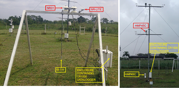
Fig. 1 Arrangements of the sensors at the meteorological site, Obafemi Awolowo University, Ile-Ife, Nigeria.
The data used for this study were measured from January 2016 to December 2017. The downward longwave radiation flux at the site was measured using an IR01 pyrgeometer of spectral response between 4.5 and 50 μm. The incoming solar radiation flux was measured with a SR01 pyranometer of spectral range between 0.3-2.8 μm. IR01 and SR01 sensors are contained in the four-component net radiometer (model NR01, Hukseflux, USA) installed at a height of 1.75 m above the ground surface (Fig. 1). The sensitivity of the net radiometer ranges from 8.2 to 15.7 µV/Wm-2 with a field view of 180º. Air temperature and relative humidity were measured using a Vaisala HMP45C probe (Campbell Scientific, USA) installed at a 2-m height (Fig. 1). The temperature sensor has an accuracy of ± 0.05 ºC. The relative humidity sensor has an accuracy at 20 ºC ± 2% (0 to 90% relative humidity) and ± 3% relative humidity (90 to 100% relative humidity). The calibration constants of the net radiometer and Vaisala probe provided by the manufacturer were used. All the sensors were recalibrated before and after measurements and no significant drift was observed in the calibration constants of the instruments after the measurement period (Soneye, 2018; Soneye et al., 2019). In this study, the cleaning of all the sensors was performed on a regular basis by cleaning their lenses and domes gently with a moistened cotton swab dipped in distilled water and alcohol to avoid the scratching of the thin optical coating on the window. The radiation shield of HMP45C was checked monthly to ensure that the radiation shield was free from debris and dust. Regarding the NR01 sensor, the interior of the dome was carefully inspected to ensure that there was no condensation, and the sensor inversion test was carried out. This sensor inversion test is a recommendation from the sensors’ manufacturer, and it involves the inversion of the position of the sensor (a 180º turn) and the checking of the output signals, which must be of the same magnitude but with a reversed sign (+ to - and - to +). For best results, this test was done on a clear day around noon when the sun was high in the sky for the pyranometers and on a clear night for the pyrgeometers. Furthermore, the cables of all the sensors were checked at regular intervals for crackings. The data was acquired using Campbell Scientific CR1000 dataloggers with sampling rate of 10 s and storage time of 1 min for further processing (Fig. 1).
2.3 Proposed model under cloudless sky conditions
An equation for estimating downward longwave radiation under cloudless sky condition (Eq. ENT#091;12SENT#093; in the supplementary material) was proposed.
2.3.1 Evaluation method
The downward longwave radiation models under cloudless sky conditions defined in Table I were evaluated. Firstly, the downward longwave radiation models with their original coefficients were tested against the measured data. Secondly, the experimental coefficients estimated at local conditions from the models were tested against the measured data. A dataset of 34 560 measurements with cloud amount ≤ 0.1, clearness index ≤ 0.13, high air temperature between 30 and 38º C and low relative humidity between 20 and 40% was used for the study. The cloud amount was determined using Eq. (S1) in the supplementary materials, which was proposed by Jegede et al. (2006). The dataset was separated randomly into two equal parts. The first half of the dataset (17 280 data) was used to test the models while the second half (17 280 data) was used to calibrate the models. The accuracies and performances of all the models before and after calibration were assessed using the statistical errors listed in Eqs. (S3) to (S11) in the supplementary materials. The calibration was done using a nonlinear least square fit to adjust the original coefficients of the models.
3. Results and discussion
The diurnal variation of clear-sky downward longwave radiation measured and estimated using original coefficients of the models is shown in Figure 2. From the time series plots, the peak values of both measured and estimated downward longwave radiation are observed to be in the late afternoon periods (usually between 15:00 and 17:00 LT) while lower values were recorded at nighttime and early morning. The values of the measured and estimated longwave radiation flux are low throughout the late evening and morning (around 21:00 to about 08:00 LT). In Figure 2 it can be seen that daytime values reach a maximum of 436 Wm-2 at 16:00 LT while the estimated values from the models reach maximum values between 378 and 505 Wm-2. The Swinbank (1963), Idso and Jackson (1969), Deacon (1970) and Prata (1996) models gave the maximum values of about 456, 461, 450 and 505 Wm-2, respectively, during daytime at 16:00 and 17:00 LT. The Ångström (1929), Brutsaert (1975), Idso (1981), Garratt (1992), Dilley and O’Brien (1998), Guest (1998), and Niemela et al. (2001) models underestimated the downward longwave radiation flux with maximum values of 411, 405, 415, 378, 382, 427 and 425 Wm-2, respectively, at 15:00, 16:00 and 17:00 LT. It was observed that the values obtained tfrom Idso (1981) and Niemela et al. (2001) models were lower and closer to the measured values. The differences in values of the downward longwave radiation estimated from all the models and direct measurements are because the coefficient of each empirical model is site-specific due to variations in the water vapor pressure and air temperature, which ensue from the temporal and spatial variations in atmospheric circulation and land use patterns, respectively (Dale, 1997; Kessler and Jaeger, 1999; Alaa et al., 2017).
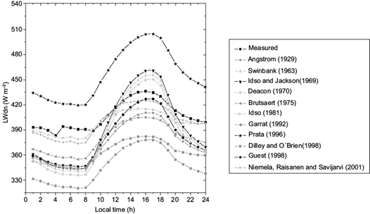
Fig. 2 Variations of the clear-sky downward longwave radiation flux (LWdn), both measured and estimated using the original coefficients of the models.
The linear regression of downward longwave radiation flux between measured and estimated values using the original coefficient is presented in Figure 3, while the performances of the models compared to measured data is presented in Table II. The analysis was done for quantitative evaluation of all the models with respect to the measured data. It was observed that the original Swinbank (1963), Idso and Jackson (1969), Deacon (1970), and Prata (1996) models overestimated the flux (Fig. 3). The overestimation of the flux by these models is affirmed by the high values of errors (MBE ~ 49 Wm-2, RMBE ~ 12%, RMSE ~ 52 Wm-2, RRMSE ~13%, MAE ~ 49 Wm-2, RMAE ~ 12%) obtained when compared to the other models. The low values obtained for the correlation coefficient and coefficient of determination of these models (~ 0.82 and ~ 0.68, respectively) indicate greater deviation and worse agreement between the values estimated from the models and the measured data. On the other hand, the original Ångström (1929), Brutsaert (1975), Garratt (1992), Dilley and O’Brien (1998), and Guest (1998) models were observed to underestimate the flux. The best results were obtained with the Idso (1981) and Niemela et al. (2001) models with low values of errors and higher values of the index of agreement (d ENT#091;see Eq. S11 in the supplementary materialsENT#093;) closer to the unity, which show good agreement between the estimated values and the experimental data. The under/overestimation of the downward longwave radiation flux by the models can be attributed to the assumption of atmospheric humidity as an implicit function of ambient temperature based on the strong correlation between water vapor pressure and air temperature by all the models (Iziomon et al., 2003). Also, the under/overestimation of the downward longwave radiation flux by the models when compared to measured values at the study site can be attributed to the differences between geographical location, cloud formation, precipitation, atmospheric turbulence and pollution levels of Ile-Ife and the various sites where all the models’ coefficients were developed (Sozzi et al., 1999; Alaa et al., 2017).
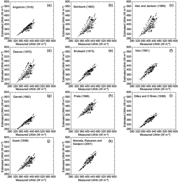
Fig. 3 Regressions between clear-sky downward longwave radiation flux (LWdn), both measured and estimated using the original coefficients of the models.
Table II Statistical results of downward longwave radiation models using their original coefficients.
| Models | R | R2 | MBE (Wm-2) | RMBE (%) | RMSE (Wm-2) | RRMSE (%) | MAE (Wm-2) | RMAE (%) | d |
| Ångström (1918) | 0.88 | 0.77 | -33.49 | -8.22 | 36.09 | 8.86 | 33.49 | 8.22 | 0.71 |
| Swinbank (1963) | 0.76 | 0.57 | -18.95 | -4.65 | 34.48 | 8.47 | 29.26 | 7.18 | 0.77 |
| Idso and Jackson (1969) | 0.76 | 0.57 | -15.08 | -3.70 | 33.37 | 8.19 | 28.17 | 6.92 | 0.79 |
| Deacon (1970) | 0.76 | 0.57 | -23.78 | -5.84 | 37.14 | 9.12 | 31.78 | 7.80 | 0.75 |
| Brutsaert (1975) | 0.92 | 0.85 | -27.50 | -6.75 | 29.96 | 7.35 | 27.45 | 6.75 | 0.79 |
| Idso (1981) | 0.89 | 0.81 | -9.33 | -2.29 | 16.78 | 4.12 | 14.43 | 3.54 | 0.92 |
| Garratt (1992) | 0.91 | 0.84 | -60.65 | -14.89 | 61.68 | 15.14 | 60.66 | 14.89 | 0.53 |
| Prata (1996) | 0.82 | 0.68 | 49.02 | 12.03 | 52.38 | 12.86 | 49.02 | 12.03 | 0.57 |
| Dilley and O’Brien (1998) | 0.93 | 0.86 | -44.92 | -11.03 | 46.12 | 11.32 | 44.92 | 11.03 | 0.63 |
| Guest (1998) | 0.83 | 0.68 | -27.04 | -6.64 | 32.39 | 7.95 | 28.59 | 7.02 | 0.76 |
| Niemela et al. (2001) | 0.92 | 0.85 | -7.43 | -1.82 | 16.46 | 4.04 | 13.65 | 3.35 | 0.93 |
d: index of agreement.
The statistical results obtained in this study compared to those reported by other authors that used the same methods is presented in Table III, where it is shown that the statistical results obtained by other authors were developed under different weather conditions from the tropical climate where this study was conducted. From the table it can be seen that the Ångström (1929), Idso and Jackson (1969), Brutsaert (1975), Prata (1996), and Dilley and O’Brien (1998) models performed better than other models despite the different weather conditions of the regions where each measurement site was located. Comparing the results in Table II with those listed in Table III, the values of the coefficient of determination obtained in this study are comparable with the range of values reported for the same type of models by Santos et al. (2011) and Alaa et al. (2017). The values of R2 and RMSE obtained for both Idso and Jackson (1969) and Prata (1996) and Swinbank (1963) are similar to those obtained by Iziomon et al. (2003), Duarte et al. (2006), Bilbao and de Miguel (2007), Lhomme et al. (2007), Alados et al. (2011), Carmona et al. (2014), and Guo et al. (2018).
Table III Statistical results of clear-sky downward longwave radiation models reported by other authors.
a: intercept; b: slope.
*Measurement sites and periods:
Niemela et al. (2001): Sodankyla, Finland, summer/winter 1997.
Iziomon et al. (2003): Bremgarten (lowland)/Feldberg (Mountain), Germany, 1991-1996.
Duarte et al. (2006): Ponta Grossa (humid region, subtropical climate), Brazil, 2003-2004.
Bilbao and de Miguel (2007): Valladolid (Mediterranean continental climate), Spain, 2001-2004.
Lhomme et al. (2007): Condori (Andean Altiplano), Bolivia, 2005.
Choi et al. (2008): Florida (humid region, subtropical climate), USA, 2004-2005.
Alados et al. (2011): Tabernas, Almería (semiarid climate), Spain, 2002.
Santos et al. (2011): Ceará State (semiarid climate), Brazil, 2005-2006.
Carmona et al. (2014): Tandil (sub-humid), Argentina, 2007-2010.
Alaa et al. (2017): Baghdad, (semi-arid/ subtropical climate), Iraq, 2014-2015.
Guo et al. (2018): 71 globally distributed sites, 2000-2006.
Table IV shows the original and calibrated coefficient values for all the models, which generally were significantly different from the original values except for the Swinbank (1963), Brutsaert (1975), and Guest (1998) models. Percentage differences of about 11% between the calibrated and original coefficients were obtained for Ångström (1929), Idso (1982), and Niemela et al. (2001) models. Hence, to improve the performances of all the models, it is very crucial to calibrate their original coefficients. The results obtained for coefficients a 5 and b 5 for the Brutsaert (1975) model are similar to those reported by Carmona et al. (2014).
Table IV Comparison of original/local and calibrated coefficient values for the 11 downward longwave radiation models under cloudless sky condition.
| Model | Coefficients | Original coefficients | Calibrated coefficients | Relative difference (%) |
| Ångström (1929) | a 1 b 1 | 0.83 0.18×10-0.067 | 0.9176 0.3355×10-0.067 | 11 |
| Swinbank (1963) | a 2 | 0.94×10⁻⁵ | 0.9774 10-5 | 4 |
| Idso and Jackson (1969) | a 3 b 3 | 0.261 -7.77×10⁻⁴ | 0.0573 -7.9073×10⁻⁶ | -78 -89 |
| Deacon (1970) | a 4 b 4 | 0.94×10⁻⁵ 0.035 | -6.0931×10⁻⁶ -4.7882 | -165 -13 781 |
| Brutsaert (1975) | a 5 b 5 | 1.24 0.143 | 1.1833 0.1014 | -5 -29 |
| Idso (1981) | a 6 b 6 | 0.7 5.95×10⁻⁵ | 0.7795 3.8700×10⁻⁵ | 11 -35 |
| Garratt (1992) | a 7 b 7 | 0.79 0.174 | 0.9408 0.2632 | 19 51 |
| Prata (1996) | a 8 b 8 | 1.2 3 | 1.8097 0.5025 | 51 -83 |
| Dilley and O’Brien (1998) | a 9 b 9 c 9 | 59.38 113.7 96.96 | 89.1642 130.9419 83.1233 | 50 15 -14 |
| Guest (1998) | a 10 b 10 c 10 | 1.0438 0.2486 113.6 | 1.0983 0.8933 147.6721 | 5 259 30 |
| Niemela et al. (2001) | a 11 b 11 | 0.72 0.009 | 0.7888 0.0059 | 10 -35 |
The statistical results of the calibrated models, and the accuracy of the models before and after calibration are presented in Table V and Figure 4, respectively. The results show that the locally calibrated models performed better than the original models (Table V and Fig. 4). As presented in Table V, the values of all statistical errors for the calibrated models were greatly reduced. The highest values of statistical errors were obtained from the models that use only air temperature (calibrated Swinbank ENT#091;1963ENT#093;, Idso and Jackson ENT#091;1969ENT#093;, and Deacon ENT#091;1970ENT#093;) despite the increase in the values of their correlation coefficient (R2 ~ 0.71) and decrease in errors (Table V, Fig. 4) when compared to the original models (R2 = 0.57). This implies that the accuracies and performances of these models are worse than the other models, which is in agreement with the results obtained by Kjaersgaard et al. (2007), Kruk et al. (2010), Carmona et al. (2014), and Guo et al., 2018. Based on the results listed in Table V, the performances of all the models are ranked as follows: Guest (1998), Dilley and O’Brien (1998), Idso (1981), Prata (1996), Brutsaert (1975), Garratt (1992), Niemela et al. (2001), Ångström (1929), Idso and Jackson (1969), Deacon (1970), and Swinbank (1963).
Table V Statistical results of downward longwave radiation models using their calibrated coefficients.
| Model | R | R2 | MBE (Wm-2) | RMBE (%) | RMSE (Wm-2) | RRMSE (%) | MAE (Wm-2) | RMAE (%) | d |
| Ångström (1918) | 0.85 | 0.72 | -1.03 | -0.24 | 15.01 | 3.43 | 11.97 | 2.74 | 0.88 |
| Swinbank (1963) | 0.84 | 0.70 | -6.20 | -1.42 | 29.80 | 6.81 | 25.58 | 5.85 | 0.74 |
| Idso and Jackson (1969) | 0.84 | 0.71 | -18.17 | -4.15 | 20.58 | 4.71 | 18.18 | 4.16 | 0.72 |
| Deacon (1970) | 0.84 | 0.71 | -17.87 | -4.09 | 20.54 | 4.70 | 17.87 | 4.09 | 0.74 |
| Brutsaert (1975) | 0.86 | 0.73 | 4.45 | 1.02 | 12.81 | 2.93 | 10.85 | 2.48 | 0.89 |
| Idso (1981) | 0.85 | 0.73 | 4.94 | 1.13 | 10.50 | 2.40 | 8.70 | 1.99 | 0.90 |
| Garratt (1992) | 0.85 | 0.73 | 2.24 | 0.51 | 13.93 | 3.19 | 11.39 | 2.60 | 0.89 |
| Prata (1996) | 0.86 | 0.73 | 4.90 | 1.12 | 12.83 | 2.93 | 10.93 | 2.50 | 0.89 |
| Dilley and O’Brien (1998) | 0.86 | 0.73 | 2.49 | 0.59 | 9.78 | 2.24 | 8.07 | 1.85 | 0.92 |
| Guest (1998) | 0.85 | 0.71 | 0.65 | 0.15 | 9.38 | 2.14 | 7.84 | 1.79 | 0.91 |
| Niemela et al. (2001) | 0.86 | 0.73 | 8.62 | 1.97 | 14.05 | 3.21 | 12.14 | 2.78 | 0.87 |
d: index of agreement.
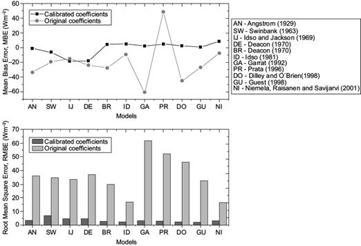
Fig. 4 Statistical measures for the downward longwave radiation flux estimated from the models before and after calibration at Ile-Ife, Nigeria.
Furthermore, the equation proposed in this study for estimating downward longwave radiation under cloudless sky conditions is expressed in Eq. (S13) in the supplementary materials. The linear regression between the downward longwave radiation flux estimated using Eq. (S13) and the measured flux is presented in Figure 5b. Also, the results of the statistical errors used to validate the proposed model and those of the best model previously tested are presented in Table VI. As shown in Figure 5a, a maximum value of about 432 Wm-2 at 17:00 LT and 434 Wm-2 at 16:00 LT were observed for the measured and estimated downward longwave radiation flux, respectively. The variations of the estimated values of the downward longwave radiation at midnight and early morning are slightly higher than the measured values. The estimated values obtained from the proposed model were observed to somehow underestimate the flux between 10:00 and 14:00 LT, and afterwards overestimate the flux until around 20:00 LT, when it coincides with the measured value. The high values of 0.93 and 0.88 obtained for the correlation coefficient and coefficient of determination, respectively, indicate great conformity and good agreement between the values estimated from the proposed model and the measured data. The results show that the performance of the proposed model is better than the performance of the all the calibrated models.
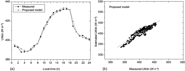
Fig. 5 (a) Diurnal variation of the clear-sky downward longwave radiation flux (LWdn), both measured and estimated from the proposed model; (b) regression between clear-sky downward longwave radiation flux (LWdn), both measured and estimated from the proposed model: 
Table VI Statistical results of the proposed downward longwave radiation model and the Guest (1998) model.
| Model | R | R2 | MBE (Wm-2) | RMBE (%) | RMSE (Wm-2) | RRMSE (%) | MAE (Wm-2) | RMAE (%) | d |
| Proposed model | 0.94 | 0.88 | -0.17 | -0.04 | 9.22 | 2.23 | 7.44 | 1.02 | 0.97 |
| Guest (1998) | 0.85 | 0.71 | 0.65 | 0.15 | 9.38 | 2.14 | 7.84 | 1.79 | 0.91 |
d: index of agreement.
4. Conclusions
Data on downward longwave radiation (long-term) are still scarce, especially in tropical regions. Most of the available empirical downward longwave radiation models were developed in areas with different climatic conditions than those of tropical regions, which is why this study evaluates and calibrates 11 existing downward longwave radiation models for clear sky conditions using meteorological data measured at Ile-Ife, Nigeria. A model for estimating clear-sky downward longwave radiation was proposed. The major conclusions derived from this study are:
The original Swinbank (1963), Idso and Jackson (1969), Deacon (1970), and Prata (1996) models overestimated the flux, while the Ångström (1929), Brutsaert (1975), Garratt (1992), Dilley and O’Brien (1998), and Guest (1998) models underestimated it.
The best results were obtained from the original Idso (1981) and Niemela et al. (2001) models, with RMBE, RMAE and RRMSE less than 5.0 %.
The performances and accuracies of all the models showed significant improvement after calibration.
The accuracies and performances of calibrated Swinbank (1963), Idso and Jackson (1969), and Deacon (1970) models, which use only air temperature as input are worse than the other models. This confirmed that other meteorological parameters such as relative humidity, precipitable water content and water vapor pressure are very important for estimating the flux under cloudless sky conditions.
The calibrated Guest (1998) model, which had low errors (MBE = 0.65 Wm-2, RMBE = 0.15%, RMSE = 9.38 Wm-2, RRMSE = 2.14%, MAE = 7.84 Wm-2, RMAE = 1.79 ) performed best, followed by the Dilley and O’Brien (1998), Idso (1981), Prata (1996), Brutsaert (1975), Garratt (1992), Niemela et al. (2001), Ångström (1929), Idso and Jackson (1969), Deacon (1970), and Swinbank (1963) models.
The proposed model had a better performance, with low statistical errors, than all the existing empirical models tested, and had a good agreement (R2 = 0.88) with the measured data. This implies that calibrating the coefficients of models developed locally is very important.
A specific model that can be used to estimate the flux over different climates in the absence of in situ data is generally unavailable.


 nueva página del texto (beta)


