


 nueva página del texto (beta)
 Inglés (pdf)
 Artículo en XML
 Referencias del artículo
 Enviar artículo por email
 Citado por SciELO
  Similares en
SciELO
Similares en
SciELO 
 Permalink
1. Introduction
Changes since 1990 in influences on the climate of Mesoamerica, including atmospheric (Liverman and O’Brien, 1991; NOAA, 2020a), ocean temperature (Méndez-González et al., 2010) and land cover (Bray, 2009) indicate that significant regional climate trends may have occurred. Predictions or explanations of the causes of climate trends or changes in these regions has often been done based on modeling of global atmospheric conditions (Karmalkar et al., 2008), ocean temperature patterns (Pounds et al., 1999), or regional land use changes (Ray et al., 2006a; Barradas et al., 2010). However, as each tropical region has its own particular topographical characteristics, oceanic influence and land cover change circumstances, the use of local data is also necessary to determine spatial details in actual regional trends and validate models.
The three physiographical regions of the Mexican state of Chiapas closest to the Pacific Ocean (subsequently referred to as Pacific Chiapas) are the Central Depression, Pacific coastal plains (Coast) and Sierra Madre de Chiapas (Sierra Madre) (Fig. 1). The climate of this area is largely influenced by large scale circulation patterns, which determine the direction of airflow, onset and length of the wet season, and frequency and intensity of rainfall events (Hewitson and Crane, 1992). The influence of these large-scale processes on regional climates may depend on trends in sea surface temperatures (SST) (Aguilar et al., 2005), which have been increasing in the Gulf of Mexico and Caribbean Sea since 1965 and 1975, respectively, in the regions closest to the east coast of Mexico (Lluch-Cota et al., 2013).
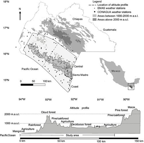
Fig. 1 Study area of the central depression, Sierra Madre, and coast regions of Chiapas, Mexico, locations of the weather stations, and an elevation profile from the Pacific Ocean to the central highlands of Chiapas. Letters S, F, T, and V indicate locations of the biosphere reserves La Sepultura (S), Frailescana (F), El Triunfo (T), and Volcán Tacaná (V).
Short term variations in temperature and precipitation patterns in Chiapas have been found to be weakly correlated with cycles of El Niño Southern Oscillation in the Pacific Ocean, although regional climate patterns varied in relation to this phenomenon (Golicher et al., 2006). Changes between the positive and negative phase of the Pacific Decadal Oscillation (PDO) could also affect climate trends during a longer time period (Méndez-González et al., 2010).
In addition to ocean temperature trends, changes in amounts of atmospheric CO2 may be influencing the climate of the region. Based on CO2 modeling, Liverman and O’Brien (1991) predicted that if CO2 doubled from the 1990 amount of 350 ppm, it would cause increases in air temperature and late dry season and summer precipitation, and decreases in precipitation at the end of the wet season and beginning of the dry season in parts of Chiapas. Since that time, atmospheric CO2 has increased to 415 ppm in 2020 (NOAA, 2020a).
Regional changes to land vegetation characteristics within Pacific Chiapas may also be influencing the mountain climate of the Sierra Madre. Modeling done on the effect of forest cover change on cloud formation in Costa Rica found that scenarios with large amounts of lower elevation deforestation resulted in lower amounts of cloud cover and higher base cloud heights in mountain forests (Lawton et al., 2001; Ray et al., 2006a). These climatic changes were largely attributed to increases in sensible heat flux from cleared land and reductions in latent heat flux due to vegetation losses (Lawton et al., 2001; Ray et al., 2006a).
Forests and dense vegetation contribute large amounts of water vapor to the atmosphere through evapotranspiration (ET) and can affect regional rainfall through recycling of ocean-source moisture (Durán-Quesada et al., 2012). Changes in vegetation can affect this process (Sheil, 2018) with reductions in tropical forest cover, generally leading to reductions in regional rainfall (Chambers and Artaxo, 2017; Casagrande et al., 2018). The main factors which control ET in an environment are vegetation density and leaf production, and climatic variables such as temperature, irradiance, wind, soil water availability, and vapor pressure (Zhang et al., 2015). In regions which are mainly covered in vegetation, such as the study area, the process of transpiration contributes to the greatest portion of ET (Ramón-Reinozo et al., 2019), although evaporation from leaf surfaces can contribute to a significant portion (Ballinas et al., 2015). In a watershed in the Sierra Madre, Castro-Mendoza et al. (2016) estimated that up to 64% of precipitation may be re-cycled to the atmosphere through ET.
Changes in vegetation cover may also affect local trends in temperature and rainfall, however the effects of this in tropical regions is still unclear. In the Lacandon rainforest in eastern Chiapas, maximum daily temperatures generally decreased in areas where there has been deforestation, but there was no relation between local rainfall and forest cover changes (O’Brien, 1998). In Guatemala, areas with greater deforestation within similar forest types had lower amounts of rainfall during the dry season (Ray et al., 2006b). The determination of links between vegetation changes and climate trends are especially important in tropical regions such as Chiapas, where land use change has been occurring rapidly (Solórzano et al., 2003).
These measured or potential changes in oceanic, atmospheric, and regional land cover conditions indicate the potential for climatic change in Pacific Chiapas. Therefore, this study examines the actual effects of these changes in large-scale and regional climatic influences on temperature and rainfall trends in this area, especially the Sierra Madre mountain range, from 1990 to 2016.
The Sierra Madre is the main source of water which flows into the Grijalva River system to produce a large quantity of Mexico’s power from dams and is an important source of freshwater resources (Jones et al., 2018). It is also a major coffee-producing region, which may be affected by changes in climate (Schroth et al., 2009). Its ecological importance has been recognized through the establishment of the biosphere reserves El Triunfo, La Sepultura and Volcán Tacaná. These reserves contain populations of flora and fauna which may be affected by long term changes (Rojas-Soto et al., 2012), or cyclical (~30-yr) trends in the mountain climate (Pounds et al., 1999; Lister and García, 2018). Various ecological studies were conducted during the establishment of the reserves in the early 1990’s (e.g., Long and Heath, 1991; Solórzano et al., 2000), and a better understanding of climatic trends since 1990 may provide a useful reference to help explain longer term ecological trends in this region (González-García et al., 2017).
The aims of this study were to determine if and where significant climate trends have occurred from 1990-2016 in Pacific Chiapas, if these were cyclical (~30-yr) or part of longer-term (~60-yr) climate changes, and how regional and larger scale processes may be influencing these trends or changes. Specifically, the first objective was to determine spatial patterns of temperature and rainfall changes and locations of significant trends from 1990-2016 in the Sierra Madre to compare with those of the adjacent lowland regions. The second objective was to determine if significant trends during the 27-yr period were part of a longer-term (1960-2016) trend in locations where data were available. The third objective was to relate climate trends to larger scale and regional climatic influence changes during similar time periods.
As mentioned, various studies have described how large-scale oceanic (Hewitson and Crane, 1992) and atmospheric processes (Liverman and O’Brien, 1991) may influence the climate of Pacific Chiapas, and we incorporated these findings into the discussion of the determined climate trends. However, to our knowledge, there have been no previous studies which have included vegetation characteristics and changes in relation to climate trends in this region. Therefore, our third objective was focused on the determination of local and regional changes in vegetation and ET from 1990-2020, which may also be influencing climate trends in Pacific Chiapas and particularly in the mountain regions.
2. Methods
2.1 Study area and time period
Pacific Chiapas (Fig. 1) is a topographically and ecologically complex region where mountainous and coastal terrain create conditions for the growth of many different forest types including mangroves, rainforests, tropical deciduous, oak-pine, cypress, fir, and cloud forests (INEGI, 2017; Fig. 1). Leaf presence is especially seasonal in the tropical deciduous forests (Gómez-Mendoza et al., 2008; Table I), but also in the more evergreen mountain forests where ET can change greatly throughout the year (Ballinas et al., 2015).
Table I Elevation range of vegetation types within the study area according to INEGI* (2017) classification, which were included in the classification of the general vegetation type.
| General vegetation type | INEGI classification | Elevation range (masl) |
| Evergreen forest (higher elevation) | Fir (Abies sp.) forest | 2000-2900 |
| Cloud forest | 700-4000 | |
| Pine forest | 500-2500 | |
| Evergreen forest (lower elevation) | Secondary tall rainforest | 200-1400 |
| Riparian forest | 600-700 | |
| Riparian rainforest | 0-700 | |
| Shade coffee plantation | Permanent agriculture | 300-2000 |
| Semi-deciduous forest | Pine-oak forest | 800-2500 |
| Oak-pine forest | 400-1900 | |
| Semi-deciduous forest | 400-1500 | |
| Oak forest | 600-1200 | |
| Fruit tree plantations | 10-25 | |
| Palm forest | 0-5 | |
| Deciduous forest | Deciduous tropical forest | 300-1700 |
| Low spiny forest | 0-10 | |
| Mangrove | Mangrove | Sea level |
| Palm plantations | Permanent agriculture | 10-50 |
| Scrub | High mountain vegetation | 3500-4000 |
| Temporary agriculture | 400-2500 | |
| Herbaceous vegetation | 550-850 | |
| Savannah | 30-800 | |
| Cleared vegetation | 50-250 | |
| Short vegetation | Irrigated agriculture | 5-700 |
| Coastal dune vegetation | Sea level | |
| Coastal wetland (Tular) | Sea level | |
| Coastal wetland (Popal) | Sea level | |
| Grassland/seasonal agriculture | Grassland | 0-1000 |
| Temporary agriculture | 0-900 |
*Instituto Nacional de Estadística y Geografía.
Similar to other regions of southern Mexico, the majority of rainfall falls between June and September (Brito-Castillo, 2012). The timing of the onset of the wet season depends strongly on the northward movement of the Intertropical Convergence Zone (ITCZ), which causes trade winds to increase in intensity and bring moist air from the Caribbean and Gulf of Mexico (Brito-Castillo, 2012). During the summer and early fall, tropical cyclones originating from the Caribbean Sea and the Pacific Ocean can bring large amounts of rainfall (García, 1974). Winter rainfall is less and is affected by cold winds originating in central North America which travel over the Gulf of Mexico, collecting humidity (García, 1974). Low pressure systems in northern Mexico also bring in moist air from the Pacific during winter (Brito-Castillo, 2012). Amounts of yearly rainfall (1990-2016 averages) are greatest in the Sierra Madre (Finca A. Prusia weather station: 2860 mm yr-1, with 85% of rainfall during the wet period from June until October), followed by the Coast (Tapachula: 2076 mm yr-1, 78% during the wet period), and lower amounts in the Central Depression (Villaflores: 1222 mm yr-1, 86% during the wet period) (Fig. 2).
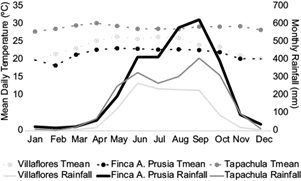
Fig. 2 Monthly averages of mean daily temperature (Tmean) and rainfall during the 1990-2016 period in the central depression (Villaflores weather station), Sierra Madre (Finca A. Prusia), and coast (Tapachula) regions.
Daytime (maximum) temperatures are highest in this region just before the wet season due to higher latent heat transfer and radiative forcing (Aguilar et al., 2005). July is often the month with the highest nighttime (minimum) temperatures due to the insulation caused by higher cloud cover (Aguilar et al., 2005). Mean daily temperatures (1990-2016 averages) are highest in the coast (Tapachula, 29 ºC), and lower at higher elevations in the Central Depression (Villaflores, 24 ºC) and the Sierra Madre (Finca A. Prusia, 22 ºC) (Fig. 2). In addition to ocean moisture sources, temperature and rainfall patterns in Pacific Chiapas are also influenced by topography and vegetation characteristics (Hewitson and Crane, 1994; Ray et al., 2006b).
Analysis of data began from 1990 to include greater spatial detail of climate trends with the inclusion of larger numbers of weather stations, which began collecting data around this year; and to provide a climatic reference for comparing ecological changes in the Sierra Madre. Comparisons of 1990-2016 trends were also done for a longer-term (57-yr) period using data from weather stations where significant 1990-2016 trends were determined and data were available since 1960.
Temperature and rainfall data were obtained from weather stations of the Comisión Nacional del Agua (National Water Commission) located within the study area (Conagua, 2018) (Fig. 1 and Table S-I in the supplementary material). Because of a lack of complete data in some weather stations and years with large amounts of cloud cover in Landsat satellite images, the analysis of land cover, NDVI, and potential ET was done using data from a range of years. Satellite images from 1987-1993 were used to represent the year 1990 and images and data from 2015-2020 to represent 2020. Rainfall and temperature trend analysis was done from 1990 to 2016 for most stations, or to 2012 or 2015 where more recent data were not available (Table S-II).
2.2 Temperature and rainfall trends
Trends and changes in average minimum (Tmin), mean (Tmean), and maximum (Tmax) daily temperature between 1990-2016 were determined using data from 55 weather stations located within the study area (Table S-I). Months were grouped into three seasons representing the main yearly changes in temperature: dry-cool (November-February), dry-hot (March-May), and wet (June-October). Temperature data for each season were obtained by averaging data of the months within each group. Differences in temperature were generally greater between months within a season than between adjacent years of the same month. Therefore, if data for a month was missing, they were estimated by calculating the average of the closest years (for up to one or two years) where data were available. This was done to avoid cooler or warmer month biases within the seasonal monthly averages where some monthly data were missing. If a station was missing more than 15% of monthly data between 1990-2016, or errors were evident (e.g., sudden breaks between temperature trend lines), it was not included in the analysis.
A graph of temperature data was done for each month and weather station and a least squares regression line was applied from 1990 to 2016. The average daily temperature value of the regression line value in 2016 was subtracted from that of 1990 to determine the change between these years. These data were uploaded into the GIS software QGIS v. 3.14 as vector points, and a spatial analysis of temperature changes was done using the Triangulated Irregular Network (TIN) method (Mitas and Mitasova, 1999) in QGIS for each season. This was chosen as the method to best represent the interpolation of the spatial changes in data which were largely influenced by topography (Velásquez et al., 2011).
Using climatic records with gaps in time series creates some uncertainty when assessing trends (Mardero et al., 2019). To correct for this, Mardero et al. (2019) interpolated data from nearby weather stations in the low elevation Yucatan Peninsula to complete rainfall records. Interpolation was also attempted in our study for stations in the Sierra Madre with missing data (Table S-II). However, results of this interpolation were inaccurate due to the large variation in rainfall between stations in the topographically complex mountain range. Therefore, the analysis of rainfall trends was done using only available data (Tables S-II and S-III).
Monthly rainfall changes between 1990 and 2016 were determined using the same method to calculate temperature changes, with data from 76 weather stations. Significant trends (p < 0.05) in temperature and rainfall were determined for three periods: 1960-1989, 1960-2016 and 1990-2016 (where data was available) using the Mann-Kendall test in the Excel extension program XLSTAT 2019. This test has commonly been used to detect significant trends in climate data. It has the assumption that data records are independent, but these data do not need to be normally distributed. As it is non-parametric, results of the test are not influenced by outlier values (Ahmad et al., 2015). Another advantage of using the Mann-Kendall test is that trends can still be determined even if a time series has missing data.
The start, end, and length of the wet season was calculated locally (rather than with regional averages) using daily rainfall data from 65 weather stations. Specifications of the start of the wet season were modified from a similar study done for the Yucatan Peninsula (Mardero et al., 2019). These were: (1) the first day of the year with measurable rainfall (≥ 1mm) followed by at least another day of rainfall within the next five days for a total of at least 20 mm of rainfall; and (2) that within the 30 days following this first day of rainfall, there was no dry spell of seven or more consecutive days without rainfall. The end of the wet season was calculated using these specifications in reverse, and the length of the wet season was calculated as the number of days between the start and the end of the wet season. Changes in the start and end of the wet season were determined by applying a regression line to a graph of the start and end dates and subtracting the values at the years 2016 and 1990 from the regression line.
2.3 Vegetation classification
Analysis of the spatial extent of forest and other vegetation cover in the years 1990 and 2020 was done to determine vegetation changes which could partially explain changes in ET, temperature, and rainfall in the study time period. The spatial extent of vegetation types was determined within the study area from the classification of Landsat level-2 atmospherically corrected images (Table S-IV). Classification was done from images captured during the dry season in order to determine vegetation types based on their density and leaf seasonality characteristics which could affect seasonal ET (Glenn et al., 2011; Ballinas et al., 2015). Images covering the study area, captured during 1987-1993 (Landsat 5) and 2017-2020 (Landsat 8) and which had less than 10% cloud cover, were downloaded from the USGS Earth Explorer website (USGS, 2020). The green, red and infrared bands (bands 2, 3, and 4 of Landsat 5, and bands 3, 4, and 5 of Landsat 8) were combined in QGIS, and these resulting images were uploaded into the land classification software Multispec v. 3.4.
Supervised classification of the image was done in this program to determine the land cover classes: evergreen forest (primary and secondary coniferous, cloud, and rainforest), mangrove, palm plantations, semi-deciduous forest (oak, pine-oak, fruit tree), deciduous forest, scrub, irrigated agriculture or short vegetation (often wetlands), grassland or seasonal agriculture, areas without vegetation (bare soil, rock, urban areas), water (lakes, rivers, coastal waters within the study area), and cloud cover (Table II). Evergreen forests, mangroves and palm plantations were determined as separate classes for areas dominated with tree cover which appeared as darker red in the combination of satellite images. As these evergreen forest types had similar spectral characteristics, images covering the coast and coastal plains were classified separately from the mountain and inland areas to avoid an erroneous classification of mangroves or palm plantations within the entire study area.
Table II Areas of vegetation types in 1990 and 2020 within the three physiographic regions of the study area (central depression, Sierra Madre, coast), and these three regions together (Pacific Chiapas). The percent of regional area of each land cover is shown next to the area values.
| Vegetation type | Year | Area (in ha) and percent (between parentheses) of each vegetation type | |||
| Central depression | Sierra Madre | Coast | Pacific Chiapas | ||
| Evergreen forest | 1990 | 43 663 (3) | 328 565 (60) | 152 917 (17) | 525 145 (19) |
| 2020 | 708 66 (6) | 351 099 (64) | 172 090 (19) | 594 055 (22) | |
| Semi-deciduous forest | 1990 | 238 366 (19) | 128 683 (24) | 144 230 (16) | 511 279 (19) |
| 2020 | 251 561 (20) | 121 921 (22) | 187 219 (21) | 560 701 (21) | |
| Mangrove | 1990 | 0 | 0 | 28 549 (3) | 28 549 (1) |
| 2020 | 0 | 0 | 36 958 (4) | 36 958 (1) | |
| Palm plantations | 1990 | 0 | 0 | 0 | 0 |
| 2020 | 0 | 0 | 7152 (1) | 7152 (<1) | |
| Deciduous forest | 1990 | 331 660 (26) | 29 575 (5) | 15 932 (2) | 377 167 (14) |
| 2020 | 258 537 (20) | 15 275 (3) | 21 178 (2) | 294 990 (11) | |
| Scrub | 1990 | 413 594 (32) | 13 193 (2) | 73 593 (8) | 500 380 (18) |
| 2020 | 453 043 (35) | 36 996 (7) | 144 389 (16) | 634 428 (23) | |
| Agriculture/short vegetation/wetland | 1990 | 31 898 (2) | 23 136 (4) | 214 166 (24) | 269 200 (10) |
| 2020 | 13 837 (1) | 6155 (1) | 116 486 (13) | 136 478 (5) | |
| Grassland/seasonal agriculture | 1990 | 168 002 (13) | 15 914 (3) | 222 593 (25) | 406 509 (15) |
| 2020 | 185 263 (14) | 10 137 (2) | 149 174 (17) | 344 574 (13) | |
| No vegetation | 1990 | 5062 (<1) | 897 (<1) | 6458 (1) | 12 417 (<1) |
| 2020 | 5828 (<1) | 928 (<1) | 16 321 (2) | 23 077 (1) | |
| Water | 1990 | 50 753 (4) | 0 | 27 839 (3) | 78 592 (3) |
| 2020 | 43 723 (3) | 0 | 30 129 (3) | 73 852 (3) | |
Semi-deciduous forest appeared as fainter dark red, deciduous forest as darker brown and scrub as lighter brown. Irrigated agriculture or wetlands appeared as lighter red or darker pink, and non-irrigated fields or soil as light grey (Fig. 3). Coastal wetland and coffee plantation subclasses were difficult to distinguish from the irrigated agriculture/short vegetation and evergreen forest classes in the satellite images. Therefore, INEGI series 6 vegetation classifications (INEGI, 2017) corresponding to these vegetation types were used to determine the spatial extent of these subclasses (Table I). Validation of the 2020 vegetation classes was done using 967 reference points randomly placed within the study area. The vegetation classification corresponding to each of these points was compared with vegetation types in higher resolution Google Earth images captured during the dry season from 2017 to 2020. Errors of commission and omission were calculated in a confusion matrix of these validation points (Table III).
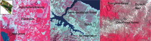
Fig. 3 Examples of vegetation types used for classification in the combination of the green, red, and infrared bands of the satellite images in the (1) coast, (2) central depression, and (3) Sierra Madre regions of Chiapas, Mexico.
Table III Confusion matrix of 967 points comparing the vegetation types classified from the 2020 Landsat images (Classification) with the validation in Google Earth (Reference).
| Classification | Reference | ||||||||||
| E | SD | D | Scrub | SV | Grass | No-V | Man | Palm | Total | Error of commission (%) | |
| E | 159 | 5 | 0 | 5 | 4 | 0 | 0 | 0 | 17 | 190 | 16.3 |
| SD | 11 | 120 | 0 | 11 | 8 | 1 | 0 | 7 | 8 | 166 | 27.7 |
| D | 0 | 11 | 61 | 12 | 0 | 2 | 0 | 0 | 0 | 86 | 29.1 |
| Scrub | 0 | 8 | 3 | 170 | 1 | 24 | 2 | 1 | 1 | 210 | 19.1 |
| SV | 2 | 2 | 0 | 3 | 93 | 1 | 0 | 3 | 2 | 106 | 12.3 |
| Grass | 0 | 1 | 0 | 8 | 1 | 126 | 1 | 0 | 0 | 137 | 8.0 |
| No-V | 0 | 0 | 0 | 0 | 2 | 0 | 9 | 3 | 0 | 14 | 35.7 |
| Man | 0 | 0 | 0 | 0 | 0 | 0 | 0 | 40 | 0 | 40 | 0 |
| Palm | 0 | 0 | 0 | 0 | 0 | 0 | 0 | 0 | 18 | 18 | 0 |
| Total | 172 | 147 | 64 | 209 | 109 | 154 | 12 | 54 | 46 | 967 | |
| Error of omission (%) | 7.6 | 18.4 | 4.7 | 18.7 | 14.7 | 18.2 | 25.0 | 25.9 | 60.9 | ||
E: evergreen forest; SD: semi-deciduous forest; D: deciduous forest; SV: irrigated agriculture/short vegetation; Grass: grassland or seasonal agriculture ; No-V: no vegetation; Man: mangrove; Palm: palm plantation.
2.4 Estimation of evapotranspiration
Various methods have been developed to estimate ET from specific vegetation types to ET at a regional scale (Fisher et al., 2011). The purpose of estimating ET in this study was not to determine the most accurate values for each vegetation type, but rather to determine the processes that have occurred in the study region which may be influencing ET, and as a result, atmospheric water vapor and orographic precipitation in the Sierra Madre. These included changes in temperature, vegetation types and cover, and seasonal changes in leaf cover which is largely influenced by rainfall patterns (Gómez-Mendoza et al., 2008).
Potential ET (PET) is a calculation of the potential amount of water vapor re-entering the atmosphere through ET from the land surface and plants (Xiang et al., 2020). This is based on mainly climatic variables, whereas actual ET is also influenced by vegetation characteristics (Allen et al., 1998). To estimate actual ET in the study area, a method incorporating PET calculations with regional vegetation index values was used (Glenn et al., 2011). This method has been used in other tropical mountain environments (Ramón-Reinozo et al., 2019).
2.4.1 Step 1
We first determined the most appropriate PET calculation method to use. The Penman Monteith (PM) method is often used as the standard to calculate PET but this requires a larger number of environmental data inputs which are not available in most weather stations in Chiapas. Previous analysis comparing the results of PET methods requiring data which are available from all stations in Chiapas with the PM method was done using data from seven weather stations of the automatic weather stations (EMAS, for their acronym in Spanish) located within or near the study area (Table S-V) (Conagua, 2020). These stations collected all the variables required for the comparisons of methods. On average, the Turc method (Turc, 1961) produced values closest to the PM value, especially in the mountain areas (Table S-V), therefore this method was chosen to calculate regional PET.
2.4.2 Step 2
PET was calculated with data from 49 weather stations within the study area. Estimations of temperature at three additional locations, based on temperatures or interpolations of temperatures recorded at nearby weather stations at similar elevations in the Sierra Madre (El Triunfo, El Porvenir; Table S-I) were also included to produce a more accurate interpolation of PET at higher elevation areas (Sierra Madre 1, 2, and 3; Table S-I). The average long-term values of Tmin, Tmean, and Tmax were calculated for each station using the value of the least squares regression line at the years 1990, 2005, and 2020. Values were calculated for these years for the same seasons as the temperature trend data: dry-cool representing the wet to dry transition season, dry-hot representing the dry season, and the wet season. PET values calculated for these years and seasons corresponded with the vegetation image layers created (described in the next steps). Raster layers of PET were created using the TIN method in QGIS.
2.4.3 Step 3
The Normalized Difference Vegetation Index (NDVI) was used as vegetation index to include vegetation characteristics in the ET estimation. Satellite images from the transition, dry, and wet seasons captured within three years of 1990, 2005, and 2020 were used to create the NDVI images (Table S-IV).
2.4.4 Step 4
A second VI formula was used to standardize the images. In the NDVI images, the most similar vegetation cover to the reference vegetation used to represent conditions where PET would be equal to actual ET was irrigated agriculture (mainly sugar cane in the Coast region) (Aguilar-Rivera et al., 2012), which had an average NDVI value of 0.82. Therefore, this value was used as the NDVI reference value (NDVIref) so that PET would be representative of the estimation of ET in this vegetation type. Denser vegetation types such as evergreen forest would have a higher estimate of ET and seasonal leaf producing vegetation types such as scrub, fields or deciduous forest during the dry season would have a lower estimate. This is representative of the natural conditions in similar mountain regions (Holwerda et al., 2013). NDVImin is the lowest NDVI value in the image. Zero was used for this value.
2.4.5 Step 5
Estimation of daily ET was then done by multiplying the PET layer obtained from the Turc calculation (step 2) and the Vegetation Index (VI) layer (step 4), which replaces the standard crop coefficient in agricultural ET estimations in order to represent natural vegetation types (Glenn et al., 2011).
INEGI series 6 polygons corresponding to the vegetation classes in this study (Table I) were used to separate ET estimations by vegetation type from the raster layers of the regional ET estimations. These raster cuts were used to estimate the mean and standard deviation of ET for each vegetation type (Table IV).
Table IV Estimations and standard deviations of evapotranspiration (ET) (mm/day) from land cover types in 1990 and 2020 during the transition from wet to dry, dry, and wet seasons.
| Land cover types | 1990 transition | 1990 dry | 1990 wet | 2020 transition | 2020 dry | 2020 wet |
| High elevation evergreen | 3.22 ± 0.52 | 3.86 ± 0.87 | 3.97 ± 0.92 | 3.04 ± 0.54 | 3.87 ± 0.77 | 3.54 ± 1.05 |
| Low elevation evergreen | 3.24 ± 0.55 | 3.69 ± 0.92 | 4.10 ± 0.75 | 3.12 ± 0.51 | 3.84 ± 0.84 | 3.89 ± 0.88 |
| Semi-evergreen forest | 2.88 ± 0.59 | 3.02 ± 0.77 | 4.05 ± 0.86 | 3.02 ± 0.55 | 3.39 ± 0.85 | 4.05 ± 0.88 |
| Shade coffee plantation | 3.52 ± 0.47 | 4.10 ± 0.72 | 4.01 ± 0.62 | 3.48 ± 0.43 | 4.26 ± 0.58 | 3.95 ± 0.94 |
| Mangrove | 3.67 ± 0.74 | 3.93 ± 0.94 | 4.05 ± 1.01 | 3.75 ± 0.66 | 4.50 ± 0.93 | 4.12 ± 0.75 |
| Deciduous forest | 2.36 ± 0.60 | 2.26 ± 0.56 | 4.02 ± 0.82 | 2.84 ± 0.59 | 2.95 ± 0.76 | 4.33 ± 0.80 |
| Scrub | 2.53 ± 0.68 | 2.63 ± 0.86 | 3.93 ± 0.75 | 2.65 ± 0.62 | 2.91 ± 0.86 | 3.99 ± 0.84 |
| Coastal wetland | 3.48 ± 0.51 | 3.43 ± 1.06 | 3.93 ± 0.66 | 3.27 ± 0.58 | 4.36 ± 0.77 | 4.29 ± 0.78 |
| Irrigated agriculture | 3.12 ± 0.84 | 2.94 ± 1.03 | 4.03 ± 0.57 | 3.12 ± 0.74 | 3.45 ± 1.10 | 3.98 ± 0.89 |
| Grassland or seasonal agriculture | 2.28 ± 0.61 | 1.99 ± 0.51 | 3.71 ± 0.84 | 2.28 ± 0.61 | 2.39 ± 0.72 | 4.01 ± 0.78 |
| Oil palm plantation | 3.76 ± 0.60 | 4.38 ± 0.92 | 4.76 ± 0.68 |
2.5 Local climate and vegetation change relations
O’Brien (1998) determined that local temperature trends were related to a higher degree with forest cover change within a radius of between 0.5 and 3 km from weather stations in the Lacandon rainforest in Chiapas, with the relationship less evident as radius sizes increased or decreased from this range. Therefore, in our study, changes in forest cover and NDVI between 1990 and 2020 during the dry season were calculated within a 2 km radius of each station where there was a significant Tmean trend. At these locations, the correlation between forest cover (evergreen, semi-deciduous, and deciduous) and NDVI changes with temperature change was tested using Spearman’s correlation test.
3. Results
3.1 Temperature trends and changes
The average Tmin in the Sierra Madre increased from 1990 to 2016 in all three seasons. In the dry-cool season Tmin increased by 0.2 ± 2.2 ºC, in the dry-hot season by 0.4 ± 1.7 ºC, and in the wet season by 0.5 ± 1.9 ºC. During the same period, Tmax decreased during the dry-cool season by 1.8 ± 1. ºC, in the dry-hot season by 1.2 ± 1. ºC, and in the wet season by 1.9 ± 1.3 ºC. The average Tmean also decreased during the dry-cool season by 0.8 ± 1.4 ºC, 0.2 ± 1.3 ºC during the dry-hot season, and 1.9 ± 1.3 ºC during the wet season.
In the lower elevation regions, there was a similar pattern with increases in Tmin during the dry-cool (coast: 1.1 ± 1.23 ºC), dry-hot (coast 1.3 ± 1.1 ºC; central depression: 0.6 ± 1.6 ºC), and wet seasons (coast: 1.5 ± 1.1 ºC; central depression: 0.7 ± 1.8 ºC). The exception was the 0.5 ± 1.6 ºC decrease in Tmin during the dry-cool season in the central depression. There was also a similar pattern to the Sierra Madre in average Tmax change with decreases in the lower elevation regions during the dry-cool (central depression: 1.6 ± 1.6 ºC), dry-hot (coast: 0.3 ± 1.1 ºC; central depression: 0.4 ± 1.9 ºC), and wet seasons (coast: 0.4 ± 1.1 ºC; central depression: 1.0 ± 1.4 ºC). There was no change in average Tmax during the dry-cool period in the coast region.
Within Pacific Chiapas, there were 48 significant trends (Mann-Kendall p < 0.05) determined for Tmean between 1990 and 2016 during the three seasons. Of these, 25 were positive (warmer) trends and 23 were negative (cooler) trends (Fig. 4, Table S-VI). Seventeen of these significant trends in temperature were from changes of 2.5 ºC or greater. Of these, five were cooler trends and 12 were warmer. Of the 10 significant temperature trends shown in the Sierra Madre, only one was warmer during the dry-hot season.
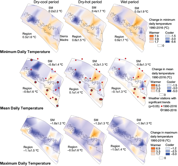
Fig. 4 Average daily temperature change between 1990 and 2016 in the central depression, Sierra Madre, and coast regions of Chiapas, Mexico. Cooler temperature changes are shown in blue and warmer changes in orange. Red points indicate locations of weather stations with significant trends in average daily temperature. The mean and standard deviation of temperature changes within the study area are written below “Region” on the map. Mean and standard deviation within the Sierra Madre (SM) region are written below “SM”.
Where data were available between 1960 and 2016, five significant earlier-period (1960-1989) trends contrasted in direction (cooler/warmer or reverse) with later- period (1990-2016) trends at the same weather station. All significant 1990-2016 temperature trends (almost all warmer) in the coast were also significant during the longer 1960-2016 period, whereas significant cooler 1990-2016 trends in the Sierra Madre were not significant during the period since 1960 (Table S-VII).
3.2 Rainfall trends and changes
There was little change in monthly rainfall in the Sierra Madre during most of the dry season from January until April. In May, which is typically at the end of the dry season, rainfall increased greatly, and this trend continued during the wet months from June until September. At the end of the wet season in October, areas within the El Triunfo and Volcán Tacaná biosphere reserves in the Sierra Madre showed dryer trends and La Sepultura, Frailescana, and the southeast region of El Triunfo, wetter trends. The months of the early dry season in November and December had average rainfall decreases between 1990 and 2016 (Fig. 5). There was a similar, but less extreme pattern of regional averages of monthly rainfall changes in the lower elevation regions, however the largest increases in rainfall occurred at the end of the wet season during the month of October (104 ± 117 mm) in the coast region (Figs. 5 and S-1).
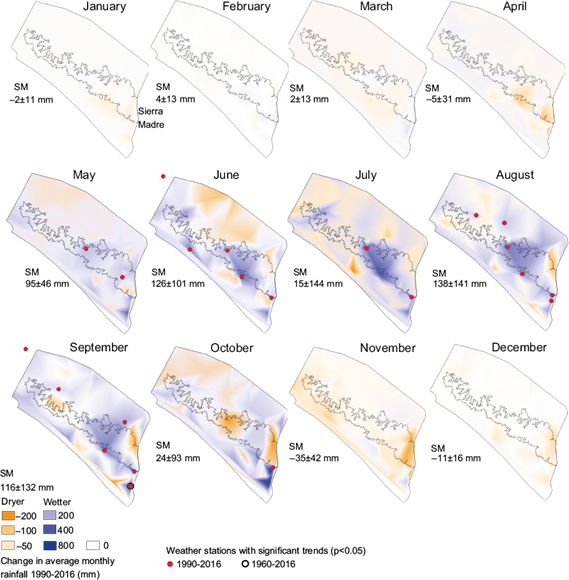
Fig. 5 Changes in monthly rainfall between 1990 and 2016 in the central depression, Sierra Madre, and coast regions of Chiapas, Mexico. Wetter changes are shown in blue and dryer changes in orange. Red points indicate locations of weather stations with significant trends in monthly rainfall. The mean and standard deviation of monthly rainfall changes within the Sierra Madre (SM) region are written below “SM” on the map.
Twenty-one significant monthly rainfall trends (Mann-Kendall p < 0.05) were determined within Pacific Chiapas. All were positive (wetter) and occurred during the months from the end of the dry season/beginning of the wet season in May until the end of the wet season in October. There were negative (dryer) trends recorded at some of the weather stations within the study area, however these were non-significant. Many of the significant trends were registered within the Sierra Madre or coastal foothills of the Sierra below 1000 m, and values of changes in monthly rainfall ranged from 110 to 650 mm. The greatest increases in monthly rainfall occurred in some of the coastal areas during the months of June and September, and in the Sierra Madre each month from June to October (Table S-III). Of these, only one significant rainfall trend was also significant during the 57-yr period from 1960-2016 at the Metapa de Domínguez weather station in the coast region, with a wetter trend for the month of September (Fig. 6, Table S-VII).
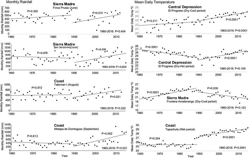
Fig. 6 Trends in monthly rainfall and mean daily temperature during the periods 1960-1989 and 1990-2016 for select weather stations in the central depression, Sierra Madre, and coast regions of Chiapas, Mexico.
The average wet season began 7.5 ± 10.6 days earlier between 1990 and 2016 in the Sierra Madre, which corresponds to the wetter trend in rainfall during May. The average end of the wet season was also earlier by 4.9 ± 8.4 days, due to dryer trends in October in some parts of the Sierra Madre. On average, the length of the wet season increased by 2.7 ± 13.6 days, although this varied greatly with the central portion of the Sierra Madre increasing, and the southeast portion near to Volcán Tacaná decreasing in length (Fig. 7). The average wet season also began earlier in the lower elevation regions (coast: 6.2 ± 13.2 days; central depression: 7.8 ± 15.1 days) but, in contrast to the Sierra Madre, ended later (coast: 1.1 ± 9.4 days; central depression: 4.2 ± 10.5 days).
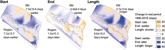
Fig. 7 Changes in the number of days between 1990 and 2016 in the start, end and course of the wet season. The mean and standard deviation of changes in days of the start, end, and course of the wet season within the entire study area (Pacific Chiapas) are written below “Region” on the map. The mean and standard deviation within the Sierra Madre (SM) region are written below “SM”.
3.3 Changes in vegetation types and evapotranspiration
The difficulty in determining boundaries between vegetation types with similar characteristics is shown in the results of the confusion matrix of the vegetation classification validation (Table III). There was an overclassification of evergreen forest within the palm plantations and mangrove types due to the similarities of these forests, especially with the 30 m2 resolution of Landsat images. There was also a higher overlap in classification of deciduous vegetation with gradients between types. The overall accuracy of the 2020 vegetation classification was 82%.
Between 1990 and 2020, the combined area of evergreen and semi-evergreen forest types (cloud forest, rainforest, oak, pine and other coniferous forests, fruit tree, palm plantations, and mangroves) increased in all three regions. In the central depression, these forest types increased by 14%, in the Sierra Madre by 3%, and in the coast by 22%; however, with the inclusion of deciduous forest as part of the overall forest areas, forest cover decreased from 1990 to 2020 in the central depression. Deciduous forest has similar characteristics than the scrub type and the boundary is not always clear in the satellite images or in the field, as there can be a gradient between deciduous tree cover and shrubby savanna. The area of scrub vegetation and grassland/temporary agriculture can also change throughout the year, as large areas of land which had grown to become scrublands are burned each year to clear land for cultivation. The combined land cover of deciduous forest or scrub decreased by 5% in the central depression but increased by 22% in the Sierra Madre and 85% in the coast (Fig. 8, Table II).
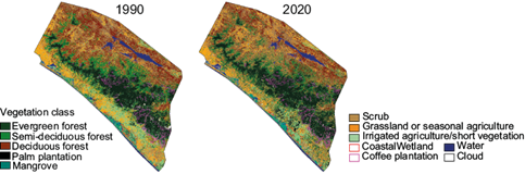
These changes in vegetation types created conditions for larger areas of leaf-covered forests in the transition and dry seasons in all regions. Leaf producing forest cover also increased in the Sierra Madre and coast regions during the wet season, but not in the central depression, where the inclusion of deciduous forests (which produce leaves in the wet season) reduced the overall area of leaf-producing forest (Fig. 9). These seasonal and long-term changes can also be seen in the average values of the NDVI (Table S-VIII), which increased in all regions for all three seasons between the 1990 and 2020 images. These increases during the wet season in the central depression could be due to denser growth of the scrub vegetation type or a lower NDVI value at the end of the wet season (November) in the 1990 image compared to the earlier date of the image captured in the 2020 wet season (August). Most of the comparisons in the period 1990-2020 (30 years) were done between similar times of the year, but there were no Landsat images during the 1987-1993 wet season without large amounts of cloud cover, so the use of an image captured in November was the best option available.
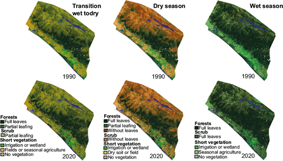
Fig. 9 Seasonal vegetation characteristics of the transition from wet to dry, dry, and wet seasons in 1990 and 2020.
This vegetation index (live green vegetation density) increases, which theoretically would create conditions for greater ET, were offset by decreases in PET between 1990 and 2016, during all three seasons. These decreases were due to the overall regional temperature changes, which were on average warming Tmin and cooling Tmax. Overall decreases in PET were outweighed by the increases in vegetation index and estimated ET increased between 1990 and 2020 from 2.70 to 2.83 mm/day in the transition season, 2.83 to 3.16 mm/day in the dry season, and without change in the wet season. However, there was variation in the direction of changes between these years with an increase in estimated ET between 1990 and 2005 and a decrease between 2005 and 2020, during the transition season. ET decreased slightly between 1990 and 2005 and then increased between 2005 and 2020 during the dry and wet seasons (Fig. 10).
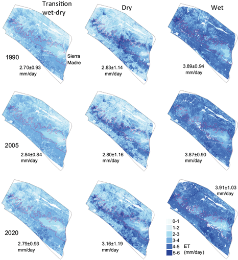
Fig. 10 Estimates of evapotranspiration in the transition from wet to dry, dry, and wet seasons of 1990, 2005, and 2020 in the Pacific regions of Chiapas, Mexico. The mean and standard deviation of evapotranspiration within the study area is written next to each image.
During the 2020 dry season, the highest amounts of ET were estimated for the coastal low-elevation evergreen vegetation types: mangrove, palm plantation, and coastal wetland (Table IV). These were followed by mountain evergreen vegetation types: shade coffee, high elevation evergreen forest, low elevation evergreen forest, and lower elevation irrigated agriculture. Lower ET were estimated for deciduous or dry vegetation types: deciduous forest, scrub, and non-irrigated land. During the wet season, when all vegetation types produce green leaves, the denser, low-elevation vegetation, including deciduous forest had the highest estimation of ET. ET decreased with vegetation types at higher, cooler elevations in the Sierra Madre. During the transition season, the highest amounts of ET were observed in the lower-elevation evergreen vegetation types, with ET decreasing in the higher-elevation evergreen types and the lowest amounts in the deciduous vegetation types as leaves dry and fall.
During the dry season, estimates of ET increased from 1990 to 2020 in all vegetation types, except the high-elevation evergreen forest where there was no change (Table IV). During the wet season, ET only increased in the lower-elevation vegetation types between 1990 and 2020 and decreased in the mid- to higher-elevation forest and coffee plantation vegetation. There was little change in the scrub type. Lower-elevation vegetation types also had increases in ET during the transition season, except for the coastal wetland which had a decrease. ET also increased in the mid-elevation semi-evergreen forest during this season. The evergreen forest types and coffee plantations in the Sierra Madre had decreases in ET.
3.4 Relation between local climate trends and vegetation changes
There was no clear correlation between vegetation changes within a 2-km radius of weather stations where there was a significant trend in Tmean, and changes in Tmean at these locations. This was the case for both changes in NDVI (p = 0.88), and percent change in forest cover (p = 0.85). Some areas which had experienced reductions in forest cover between 1990 and 2020 had positive trends of Tmean, whereas others had negative trends. Likewise, areas that experienced gains in forest cover had either positive or negative Tmean trends.
4. Discussion
4.1 Comparisons between 1960-2016, 1990-2016 trends and large-scale climatic influences
The generally wetter wet seasons and dryer dry seasons during the 1990-2016 period in all three regions were consistent with global trends in precipitation (Murray-Tortarolo et al., 2017) during a similar time period (1980-2005). Murray-Tortarolo et al. (2017) discussed that these trends may have been the result of global oceanic (La Niña years) and atmospheric (1991 Mt. Pinatubo eruption) conditions during the late 1980s and early 1990s, which lowered global precipitation during these years, and the beginning of global warming influences. However, the relation between rainfall and La Niña are variable within Mexico and are generally associated with higher rainfall in Southern Mexico (Bravo-Cabrera et al., 2017). The lack of significant trends in rainfall in Pacific Chiapas during a longer time period (1960-2016) at most weather stations where there was a wetter trend during the 1990-2016 period, was also consistent with global trends (Murray-Tortarolo et al., 2017), except for an area of the Coast (Metapa de Domínguez during September; Fig. 5, Table S-VII) where there was an extended 57-yr significant wetter trend.
Significant cooler trends between 1990-2016 in the Sierra Madre were not significant since 1960, which contrasted with the longer continuation of significant warmer trends in the coast. Increasing trends in rainfall since 1990 in the mountain region may be related to the cooler trends during 1990-2016 (mostly due to decreases in Tmax; Fig. 4) at higher elevations because of greater cloud cover.
Regional climatic trends between 1990 and 2016 in Pacific Chiapas were consistent with those attributed to the effects of long-term trends in the Pacific Decadal Oscillation (PDO) in southern Mexico (Méndez-González et al., 2010). During this period, the PDO index showed a negative trend from a positive phase in the 1990s to a negative phase in the 2000s (NOAA, 2020b). Méndez-González et al. (2010) determined that from 1950-2007, negative periods of the PDO have been associated with higher summer precipitation, cooler summer Tmax, and warmer Tmin in southern Mexico. These trends were determined on average for the study region, although not consistently for all weather stations, especially in some parts of the coast, which had increases in both Tmin and Tmax (Fig. 4).
Summer rainfall in Chiapas is also strongly influenced by the ITCZ bringing moisture from the Caribbean Sea and Gulf of Mexico. SSTs have increased both in the Gulf of Mexico and the Caribbean since 1975 (Lluch-Cota et al., 2013), and higher amounts of evaporation from a warmer surface may increase atmospheric moisture and intensify downwind rainfall (Brito-Castillo, 2012). Increases in rainfall often indicate cloudier conditions and this can affect regional temperatures (Englehart and Douglas, 2005), effects consistent with the determined regional trends. Increased cloud cover blocks incoming day time solar radiation, lowering Tmax, whereas nighttime Tmin are increased by the insulation of cloud cover, which reemits longwave radiation back to the ground. The predicted climate effects of increases in global atmospheric CO2 from 1990 amounts described by Liverman and O’Brien (1991) for the southern Pacific region of Mexico were also consistent with those determined by this study for rainfall patterns, although the predicted temperature increases were only determined on average for Tmin.
4.2 Relations between land use change, vegetation and climate trends
Between 1970 and 2000, Chiapas experienced large amounts of deforestation (Richter, 2000; Solórzano et al., 2003). However, reviews published in the years after 2000 began to discuss a possible change in the rate of deforestation and beginning of reforestation in parts of Mesoamerica (Bray, 2009). Evidence supporting this prediction may be shown by Vaca et al. (2012), who reported a decreased annual rate of deforestation between the periods of 1990-2000 and 2000-2006 in the dry tropical forests of the central depression of Chiapas. Bonilla-Moheno and Aide (2020) also reported an increase in forest cover in the lower elevation, inland portion of the Sierra Madre between 2001-2014, which was consistent with what was determined in this study.
The abandonment of agricultural areas during increased urban migration, and the large scale of land which had already been deforested by 1990 may have contributed to increased forest cover in the areas adjacent to the Sierra Madre between 1990 and 2020 (Bonilla-Moheno and Aide, 2020). Trends of increasing rainfall in these regions may also have been influential for regeneration of forests in abandoned agricultural areas, even when there were large variations in rainfall between years (Martínez-Ramos et al., 2018). The steep and less accessible Sierra Madre region was by far the most forested of the study area, with very little overall change in forest cover. The establishment of biosphere reserves beginning in 1990, and programs such as Payment for Hydrological Environmental Services within communities of the Sierra Madre influenced the slower changes in this region (Cano-Díaz et al., 2015).
Large differences in species composition can exist between vegetation types which are difficult to distinguish remotely, such as regenerating deciduous forests and native scrub ecosystems (Gordillo-Ruiz et al., 2020). Species composition, diversity and succession stage can influence differences in vegetation responses to climate trends and ET (Ballinas et al., 2015; Sakschewski et al., 2016). Additionally, topography, vegetation cover, and soil characteristics of landscapes can influence water availability from rainfall (Ponette-González et al., 2010; Schwartz et al., 2019); and vegetation can have physiological responses to changes in climate allowing them to regulate ET (Massmann et al., 2019). These physiographic and physiological characteristics indicate a limitation of the modeling we used to estimate ET. We hope our regional focus inspires further field-based studies of ET in the specific vegetation types we have included. However, the use of local climatic data and remote sensing, which showed increases in dense vegetation cover and regional estimations of ET between 1990 and 2020, were useful to understand the contribution of vegetation changes to the climate of Pacific Chiapas, in particular the coastal mountains.
Regional increases in forest vegetation and ET may have contributed to positive climatic feedback, which combined with the influences of increasing SST in the east coast of Mexico, a negative phase of the PDO in the west coast, and increasing atmospheric CO2, produced larger positive trends in rainfall during the late dry and wet seasons. Estimates of ET mainly decreased in the mountain evergreen forests between 1990 and 2020 (Table IV) due to decreasing trends in temperature (Fig. 4). However, there were overall increases in estimated regional ET, due to increases in the density of leaf producing vegetation cover and some regional temperature increases, especially in the lower elevation regions (Fig. 10, Table S-VIII). There is also a strong relationship between the onset of the wet season and the production of leaves in deciduous and semi-deciduous vegetation in Mexico (Gómez-Mendoza et al., 2008). The earlier trend in the start of the wet season in this region may indicate that leaf production is beginning earlier in the year; also that, along with increases of available soil moisture, it could result in earlier increases in ET, contributing to higher atmospheric moisture and higher orographic rainfall in the Sierra Madre.
Increases in semi-deciduous and evergreen forest cover between 1990 and 2020 may cause greater regional latent heat flux, decreases in sensible heat flux (Ray et al., 2006a, b), and increases in surface roughness (Spracklen et al., 2018). This may affect heights of orographic cloud cover, which potentially could decrease with these land cover change conditions (Lawton et al., 2001; Fairman et al., 2011), and affect the altitudinal distribution of rainfall (Barradas et al., 2010). The constant burning of regenerating deciduous forest and savannahs for seasonal agriculture in the central depression creates conditions of higher surface albedo, which can negatively affect rainfall (Fuller and Ottke, 2002). This may be another reason for the lower regional increases in rainfall in the central depression in comparison with the much greater forested Sierra Madre region.
At various locations, significant climate trends differed from the overall average regional changes (Figs. 4 and 5; Tables S-III and S- VI). There were no clear relations between local significant temperature or rainfall changes and vegetation changes (forest cover or NDVI). This suggests that the regional climate changes determined were influenced to a greater extent by long term atmospheric and oceanic processes and regional vegetation changes. Local differences in temperature and rainfall patterns may be due to topography, air flow patterns, and the orographic nature of precipitation in this mountainous region, as in other parts of Mesoamerica (Barradas et al., 2010; Maldonado et al., 2018).
Many of the ocean influence patterns are cyclical at a time scale greater than the study period of 27 years (Fuentes-Franco et al., 2015). Therefore, the climate trends and patterns determined in this study may change as trends change in the large-scale climatic influences which affect Chiapas (Aguilar et al., 2005). However, if increasing vegetation cover trends continue in this region, they may moderate future climate cycles in the Sierra Madre (Lawton et al., 2001; Bonan, 2008).
5. Conclusion
Regional 1990-2016 climate trends within Pacific Chiapas included increases in Tmin, decreases in Tmax, an earlier shift in the wet season, and greater amounts of rainfall within this season. All significant temperature trends continued from 1960-2016 in the coast region but less so in the central depression and did not in the Sierra Madre. Only one significant rainfall (wetter) trend continued during this 57-yr period, in an area of the coast. The more recent (1990-2016) trends occurred during a period of change in ocean and atmospheric climatic influences in the region, including a negative trend in the PDO index, warming SST in the Gulf of Mexico and the Caribbean, and rising amounts of atmospheric CO2. During the same time period, regional extents of evergreen and semi-evergreen forest types, NDVI values, and estimates of ET increased. These changes may have enhanced the climatic patterns influenced by large-scale processes.


