


 nueva página del texto (beta)
 Inglés (pdf)
 Artículo en XML
 Referencias del artículo
 Enviar artículo por email
 Citado por SciELO
  Similares en
SciELO
Similares en
SciELO 
 Permalink
INTRODUCTION
In recent years, the Ecological Network Analysis (ENA) has been used for evaluating ecosystem dynamics and identifying properties that are not evident from direct observation (Fath et al., 2007). Supported by analysis of trophic interactions, it is possible to estimate ecosystem properties that define aspects concerning structure, health, and dynamics of the ecosystems (Ulanowicz, 1986; Tennenbaum & Ulanowicz, 1988) and identify species or functional groups more sensitive to disturbances (Walters et al., 1997). There are at least two theoretical frameworks that analyze the ecosystem properties: (1) Odum (1969) states that the maturity of the ecosystems is approached in the maximization of the structure and function of the ecosystem, and (2) Ulanowicz (1997), carried out a theoretical framework named Ascendency which analyses the ecosystem properties such as the level of development and organization of the ecosystems based on the information theory.
Likewise, with the network analysis, it is possible to evaluate the propagation of instantaneous direct and indirect effects (Walters et al., 1997) and the magnitudes in system recovery time (SRT), a resilience measure. The above is in response to a simulated disturbance that increases the total mortality of each functional group (Ortiz et al., 2015). In this study, resilience has been conceptualized as the speed at which the entire system returns to its original state after it has been displaced from it (Pimm, 1982).
The Mexican Tropical Pacific coast presents shallow reefs and coral communities, considered the most important in the eastern Pacific (Reyes-Bonilla, 2003). Due to their location, these reefs face local stressors such as tropical storms, hurricanes, El Niño-Southern Oscillation (ENSO), and anthropogenic disturbances highlighting fisheries, tourism, sedimentation, and coastal development (Martínez-Castillo et al., 2020). Therefore, determining ecosystem properties is a potential tool for studying and evaluating the ecosystems’ structure and functioning and the capacity to face these disturbances (Heymans et al., 2014).
This work aimed to build a trophic model representing the shallow rocky-reef ecosystem in Yelapa, México to evaluate the ecosystem’s structure, organization, and maturity. In addition, it determines the species and functional groups that are most affected in response to disturbances simulated and that generate less resilience in the ecosystem. A better understanding of the ecosystemic functioning would greatly help prioritize species or functional groups that could preserve the ecosystem’s structural integrity in shallow and mesophotic ecosystems in the face of different climate change events. This study represents the first step in analyzing the trophic network properties and ecologically relevant species of shallow rocky-reef ecosystems in Yelapa.
MATERIALS AND METHODS
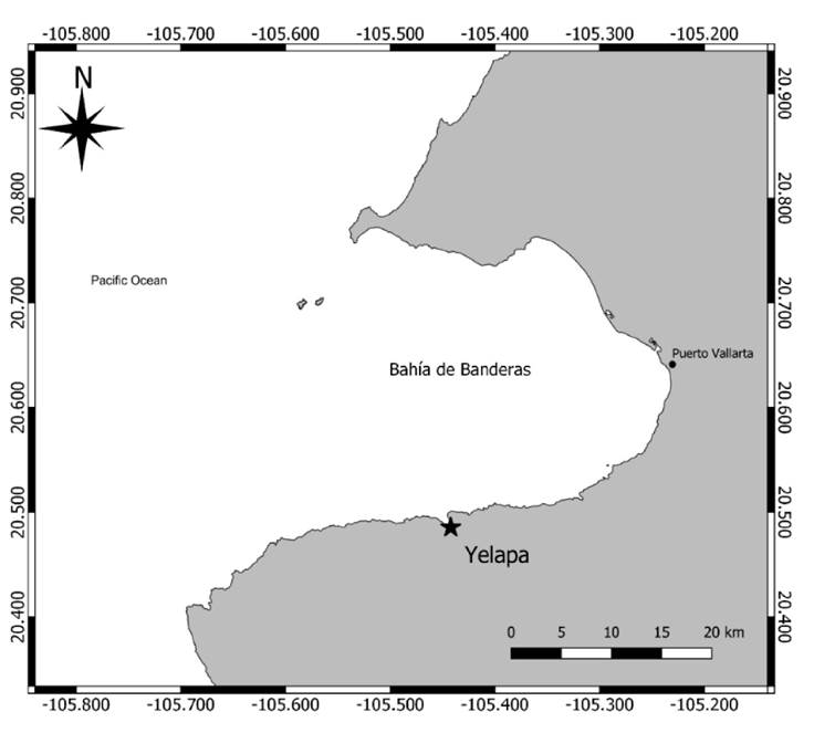
Study area. Yelapa is located south of Bahía de Banderas at the southeastern end of the Gulf of California on the Pacific coast of Mexico (Fig. 1). This bay is considered a transition zone because of the different currents that converge there. The oceanic circulation is influenced by the water masses of the California Current, the Gulf of California, the Costa Rica Current, and the North Equatorial Current that interact in this transitional region (Portela et al., 2016). In addition, the south of the bay receives freshwater from the rivers Chimo, Yelapa, and Pizota and, together with upwelling events, trigger values high in nutrients during the spring (Cotler et al., 2010). Yelapa is a small town with tourist and fisheries activities, mainly during spring and summer.
Mass balance models. Trophic models were constructed using Ecopath with Ecosim (v.6.6.1; Table 1). Ecopath allows for depicting the flows of matter and energy in a stationary state in an ecosystem within a given time. In contrast, Ecosim performs dynamic simulations of the initial conditions established with Ecopath as a response to perturbations. See details in Christensen & Walters (2004).
Table 1 Algorithms of macroscopic network properties.
| Ecosystem properties | Algorithms |
|---|---|
| Total System Throughput (TST) (g m-2 year-1 ) |
|
| Average Mutual Information (AMI) |
|
| Ascendency (Flowbits) |
|
| Total Capacity (Flowbits) | C=A+O |
| Overhead (Flowbits) | O=C-A |
Details in: Ulanowicz (1986, 1997)
Source of data. Sampling surveys were conducted in May and November 2021 by underwater visual censuses (SCUBA divers) at three sites to identify the species of the shallow benthic ecosystem. First, the abundance of fish and mobile invertebrates (crustaceans, echinoderms, and mollusks) was estimated using five belt transects (4 × 25 m) to identify species and count the number of individuals of each species. Next, those same transects were used to estimate coral cover, sessile invertebrates, and macroalgae cover (Chlorophytes and Rhodophytes) through six quadrants in each transect.
Selection of functional groups and diet matrix. A total of 91 species were recorded. The trophic model was composed of 35 functional groups and represented by both individual species and functional groups, characterized by commercial importance, their representativeness as species of these ecological systems, food preferences, and trophic relationships (Fig. 2). For each compartment, the average biomass (B), turnover rate Production/Biomass (P/B), consumption rate Consumption/Biomass (Q/B), capture (Ca), and food sources were determined from field observations and scientific sources (Table 2). When appropriate, the functional groups were trophic related to feeding on detritus, considered a source of energy and nutrients to living organisms (Moore et al., 2004).
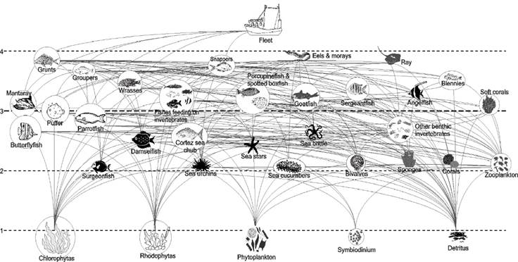
Figure 2 Trophic network of the shallow rocky reef of Yelapa, Jalisco, Mexico. The circle size is proportional to the functional group biomass (g wet weight m-2). The dotted lines correspond to the trophic levels.
Table 2 Parameter values of Ecopath models for the rocky reef ecosystem of Yelapa, where B= biomass [g m−2], P/B= turnover rate [year−1], Q/B= consumption rate [year−1], EE= ecotrophic efficiency [dimensionless], GE= gross efficiency [year−1], NE= Net Efficiency [dimensionless], RA/AS= Respiration/Assimilation [dimensionless], RA/B= Respiration/biomass [year−1], and P/RA= Production/Respiration [dimensionless].
| Group name | B | P/B | Q/B | EE | GE | NE | RA/AS | RA/B | P/RA | |
|---|---|---|---|---|---|---|---|---|---|---|
| 1 | Manta ray | 22.8 | 3.6 | 17.1 | 0.0 | 0.2 | 0.3 | 0.7 | 10.1 | 0.4 |
| 2 | Grunts | 9.4 | 2.3 | 7.8 | 0.7 | 0.3 | 0.4 | 0.6 | 4.0 | 0.6 |
| 3 | Groupers | 10.6 | 0.6 | 8.5 | 0.6 | 0.1 | 0.1 | 0.9 | 6.2 | 0.1 |
| 4 | Snappers | 9.5 | 2.4 | 10.0 | 0.6 | 0.2 | 0.3 | 0.7 | 5.6 | 0.4 |
| 5 | Wrasses | 33.2 | 2.5 | 13.1 | 0.5 | 0.2 | 0.2 | 0.8 | 7.9 | 0.3 |
| 6 | Fishes feeding on invertebrates | 8.6 | 4.5 | 15.3 | 0.5 | 0.3 | 0.4 | 0.6 | 7.7 | 0.6 |
| 7 | Porcupinefish & spotted boxfish | 3.3 | 2.4 | 10.4 | 0.4 | 0.2 | 0.3 | 0.7 | 5.9 | 0.4 |
| 8 | Goatfish | 8.8 | 2.3 | 7.8 | 0.5 | 0.3 | 0.4 | 0.6 | 4.0 | 0.6 |
| 9 | Eels & morays | 1.3 | 0.6 | 5.7 | 0.2 | 0.1 | 0.1 | 0.9 | 3.9 | 0.2 |
| 10 | Ray | 3.7 | 3.6 | 15.2 | 0.0 | 0.2 | 0.3 | 0.7 | 8.6 | 0.4 |
| 11 | Sergeant fish | 5.3 | 2.2 | 18.7 | 0.4 | 0.1 | 0.1 | 0.9 | 12.8 | 0.2 |
| 12 | Angelfish | 4.5 | 3.2 | 17.4 | 0.4 | 0.2 | 0.2 | 0.8 | 10.7 | 0.3 |
| 13 | Butterflyfish | 3.1 | 2.2 | 18.7 | 0.4 | 0.1 | 0.1 | 0.9 | 12.8 | 0.2 |
| 14 | Puffer | 15.5 | 2.4 | 12.3 | 0.4 | 0.2 | 0.2 | 0.8 | 7.4 | 0.3 |
| 15 | Parrotfish | 7.0 | 3.0 | 12.6 | 0.8 | 0.2 | 0.3 | 0.7 | 7.1 | 0.4 |
| 16 | Damselfish | 14.0 | 2.8 | 14.5 | 0.4 | 0.2 | 0.2 | 0.8 | 8.8 | 0.3 |
| 17 | Cortez sea chub | 2.5 | 2.4 | 12.3 | 0.3 | 0.2 | 0.2 | 0.8 | 7.4 | 0.3 |
| 18 | Surgeonfish | 11.3 | 3.2 | 17.4 | 0.8 | 0.2 | 0.2 | 0.8 | 10.7 | 0.3 |
| 19 | Blennies | 7.0 | 2.2 | 18.7 | 0.3 | 0.1 | 0.1 | 0.9 | 12.8 | 0.2 |
| 20 | Sea urchins | 41.5 | 7.5 | 25.0 | 0.6 | 0.3 | 0.4 | 0.6 | 12.5 | 0.6 |
| 21 | Sea stars | 7.4 | 6.5 | 23.2 | 0.4 | 0.3 | 0.4 | 0.6 | 12.1 | 0.5 |
| 22 | Sea cucumbers | 1.8 | 6.2 | 22.2 | 0.0 | 0.3 | 0.3 | 0.7 | 11.6 | 0.5 |
| 23 | Brittle stars | 11.4 | 6.5 | 23.2 | 0.3 | 0.3 | 0.4 | 0.6 | 12.1 | 0.5 |
| 24 | Other benthic invertebrates | 297.0 | 4.2 | 14.2 | 0.8 | 0.3 | 0.4 | 0.6 | 7.2 | 0.6 |
| 25 | Bivalves | 48.0 | 4.8 | 18.0 | 0.5 | 0.3 | 0.3 | 0.7 | 9.6 | 0.5 |
| 26 | Sponges | 47.2 | 3.6 | 16.4 | 0.5 | 0.2 | 0.3 | 0.7 | 9.5 | 0.4 |
| 27 | Hard corals | 63.9 | 4.4 | 16.8 | 0.4 | 0.3 | 0.3 | 0.7 | 9.1 | 0.5 |
| 28 | Soft corals | 41.9 | 3.0 | 15.5 | 0.5 | 0.2 | 0.2 | 0.8 | 9.4 | 0.3 |
| 29 | Zooplankton | 278.6 | 24.3 | 81.0 | 0.7 | 0.3 | 0.4 | 0.6 | 40.5 | 0.6 |
| 30 | Chlorophyta | 2117.7 | 6.0 | 0.1 | ||||||
| 31 | Rhodophyta | 817.2 | 6.0 | 0.2 | ||||||
| 32 | Phytoplankton | 486.1 | 57.9 | 0.8 | ||||||
| 33 | Symbiodinium | 6.3 | 238.0 | 0.7 | ||||||
| 34 | Detritus | 88.5 | 0.0 |
Source data: Opitz (1993); Aliño et al. (1993); Cruz-Romero et al. (1993); Okey et al. (2004); Liu et al. (2009); Croll et al. (2012); Frausto-Illescas (2012); Castañeda-Rivero (2017); Hermosillo-Núñez et al. (2018); Calderon-Aguilera et al. (2021).
For the construction of the diet matrix, the information was obtained from the literature (e.g., Sampson et al., 2010; Flores-Ortega et al., 2014; Hermosillo-Núñez et al., 2018; Calderon-Aguilera et al., 2021; Reyes-Ramírez et al., 2022) from studies carried out in sites close to the location of this study. It is important to mention that a recent study has showed that interaction matrices based on stomach content analysis is enough robust for assessing the trophic complexity and macroscopic properties (Ortiz, 2018).
Balancing model. The model was balanced based on the six criteria proposed by Heymans et al. (2016). The pedigree routine was used to assign the ranges of percent uncertainty of the input parameters (B, P/B, Q/B, diet, and catch values). Using the Pedigree module and the provenance of the data, the pedigree has been calculated of the model in 0.231.
Macroscopic network properties. (1) Total Biomass/Total System Throughput (TB/TST) ratio suggests different states of system maturity (Christensen, 1995); (2) Total System Throughput (TST) indicates the total number of flows in the system; (3) Average Mutual Information (AMI) quantifies the organization of the system concerning to the number and diversity of interactions between components (complexity); (4) Ascendency (A) measures the growth and development of a system; (5) Overhead (Ov) quantifies the degrees of freedom preserved by the network and can be used to estimate the ability of a network to withstand perturbations; (6) Development Capacity (C), the upper limit of Ascendency; (7) the ratios of A/C and Ov/C are used as indicators of ecosystem development and the ability of the system to resist disturbances (Kaufman & Borrett, 2010). The algorithms of network properties are shown in Table 1; (8) The connectance index (CI) measures the network structure and determines the number of trophic links; (9) The system omnivory index (SOI) shows how feeding interactions are distributed between trophic levels (Mukherjee et al., 2019); (10) Finn’s cycling index (FCI) measures the amount of material or energy cycling in ecosystems (Finn, 1980); (11) Finn’s mean path length (APL) describes how many times a unit of energy will be transferred between functional groups. In mature ecosystems, both the diversity and cycling increase; therefore, the path length is expected to increase; finally, (12) the mean trophic level of the catch (TLC) shows the trophic level at which fishing is performed.
Mixed trophic impact and dynamic simulations. The mixed trophic impact (MTI) is an Ecopath routine used to indicate the direct and indirect effects in a steady-state system; for more details, see Ulanowicz & Puccia (1990). In addition, Ecosim permits the generation of dynamical biomass predictions of each functional group i, which is affected directly and indirectly by different disturbances; for more details, see Walters et al. (1997).
The scenarios. The fishing mortality was modified to simulate an increase in the total mortality of each functional group (Z = M+F). The modifications were done between the 2nd and 9th year of the total simulation (20 years). The total mortality was increased by 25 % and 50 % from the baseline to create a situation where all functional groups are depleted. These two scenarios were set for prediction as a measure of confidence (for more details, see Ortiz et al., 2015). For the two scenarios, the dynamical simulations were done in both short-term (transient) and long-term (persistent) changes in biomass; this is the disturbances in the trophic network can be instantaneous such as fisheries or massive mortality, and persistent such as pollution, or El Niño-Southern Oscillation event (ENSO). The propagation of short-term (transient) and long-term (persistent) changes in biomass was evaluated in the 3rd and 10th year of simulation, that is, one year after the increase in mortality. All dynamic simulations by Ecosim were performed using a mixed-flow control mechanism (n = 0.3) (both prey and predators control the flow), which is considered more realistic than a bottom-up (prey control the flow) or top-down (predators control the flow) control (Muhly et al., 2013). Although no verification of the simulations using time-series calibration was conducted, this absence was mitigated by comparing different scenarios based on two levels of total mortality by functional groups (Ortiz et al., 2015).
System recovery time (SRT). The SRT is the magnitude or time at which the ecosystem returns to its original state after it has been displaced from this (a proxy to resilience) in response to a simulated disturbance that increases the total mortality (Z) of all functional groups (Ortiz et al., 2015). The SRT was evaluated using the same scenarios of disturbances as the dynamic simulations Ecosim.
RESULTS
Chlorophyta contributed the highest biomass values (Table 2). Energy flows between trophic groups in the ecosystem were expressed as Lindeman spine. The ecosystem of Yelapa showed nine theoretical trophic levels, and the main flows occurred in the first three (Fig. 3, only displayed from I to V because the flows from VI to X contributed minimally). The trophic levels II, III, and IV accounted for 35.8 % of the trophic efficiency. Flows from primary producers with biomass of 3 427 t km2 account for 26 838 t km2 year-1. The flows from detritus accounted for 641.6 t km2 year-1, suggesting that low trophic level support the Yelapa food web.
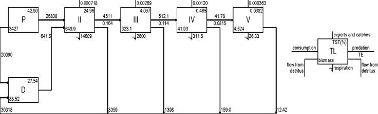
Figure 3 Lindeman spine of the rocky reef in Yelapa, showing all the trophic flows. Numbers in Roman are discrete trophic levels. P= Productors; D=: Detritus; TST=: Total system throughput; TE=: Transfer efficiency (annual).
Concerning network properties, Yelapa showed features of an organized and mature system based on the values of ecosystem properties such as total system throughput (TST), the total biomass/total system throughput (TB/TST), Ascendency (A), overhead (Ov), development capacity (C), Overhead/Capacity (Ov/C), ascendency/capacity (A/C), average mutual information (AMI), Finn’s cycling index (FCI), mean trophic level of the catch (TLC), connectance index (CI), system omnivory index (OI), and path length (APL) (Table 3).
Table 3 Network properties of Yelapa compared with localities in the Mexican Pacific, and the Gulf of California. FG= Functional Groups.
| Yelapa (34 FG) | Isabel Island (30 FG) | Marietas Island (27 FG) | Chamela (23 FG) | Cabo Pulmo (57 FG) | |
| Total system throughput (TST) (g ww m-2 year-1) | 111,657.40 | 194,758.40 | 108,102.70 | 54,977.23 | 95,789 |
| Total biomass/total system throughput (TB/TST) | 0.040 | 0.039 | 0.037 | 0.028 | 0.005 |
| Ascendency (A) (total) (Flowbits) | 169,298 | 308,428.70 | 170,017.80 | 79,678.40 | 123,662 |
| Overhead (Ov)(total) (Flowbits) | 265,844 | 581,872.90 | 306,704.50 | 162,864.10 | 116,164 |
| Development Capacity (C) (total) (Flowbits) | 435,142 | 890,301.60 | 476,722.30 | 242,542.60 | 239,826 |
| Ov/C (%) | 61.09 | 65.35 | 64.33 | 67.14 | 48 |
| A/C (%) | 38.91 | 34.64 | 35.66 | 32.85 | 52 |
| Average Mutual Information (AMI) bits) | 1.52 | 1.58 | 1.57 | 1.44 | - |
| Finn’s cycling index (FCI) (%) | 1.66 | 1.32 | 1.23 | 1.19 | 0.124 |
| Mean trophic level of the catch (TLC) | 3.40 | 3.44 | 3.47 | 3.57 | - |
| Connectance Index (CI) | 0.197 | 0.246 | 0.260 | 0.302 | 0.167 |
| System Omnivory Index (OI) | 0.218 | 0.200 | 0.250 | 0.257 | 0.218 |
| Finn’s mean path length (APL) | 2.364 | 2.624 | 2.632 | 2.637 | 2.114 |
Regarding the contribution of each compartment to the total Ascendency, the principal contributing components was detritus (32 %), followed by phytoplankton (23.1 %), zooplankton (12.9 %), and chlorophyte (12.6 %). In addition, the functional group’s eels & morays (0.006 %), Cortez Sea chub (0.029 %), and sea cucumbers (0.030 %) contributed to the system complexity (lowest % of AMI; Table 3).
The outcomes of the propagation of the direct and indirect effects estimated using Mixed Trophic Impacts (MTI) showed that functional groups of grunts, groupers, snappers, wrasses, zooplankton, and phytoplankton produced the most remarkable trophic effects in the remaining functional groups (Fig. 4).
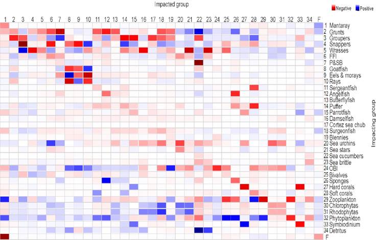
Figure 4 Propagation of the direct and indirect trophic effects estimated using Mixed Trophic Impacts (MTI) and produced by several functional groups on the remaining functional groups. FFI= Fishes feeding on invertebrates; P&SB= Porcupinefish & spotted boxfish; OBI= Other benthic invertebrates.
The Ecosim dynamic simulations showed that the phytoplankton, Chlorophyta, and other benthic invertebrates propagated more effects to other model components, using the two mortality scenarios (25% and 50%) and both short and long-term dynamic simulations (Table 4). In addition, rhodophyte and sea urchins propagated high effects on the rest of the functional groups when the disturbance was done in a short time using the two mortality scenarios. Meanwhile, snappers and wrasses generated the highest effects on the other model functional groups over a long-time and using the two mortality scenarios (Table 4). As a measure of resilience, SRT values indicated that when the snappers, eels & morays, other benthic invertebrates, and phytoplankton functional groups are disturbances, the Yelapa shallow coral ecosystem is less resilient using the two mortality scenarios and mainly long-term dynamic simulations (Table 4).
Table 4 Ecosim simulations (E) and System Recovery Time (SRT) (years) values for the shallow coral ecosystem in Yelapa using mixed control mechanism and two increments of mortality (25% and 50%).
| Increase in mortality | |||||||||
| Short-time 25% | Short-time 50% | Long-time 25% | Long-time 50% | ||||||
| Yelapa | SRT | E | SRT | E | SRT | E | SRT | E | |
| 1 | Mantaray | 10.0 | 1.5 | 12.8 | 3.1 | 20.0 | 1.9 | 23.1 | 4.7 |
| 2 | Grunts | 11.2 | 2.4 | 12.2 | 4.3 | 21.2 | 5.1 | 23.1 | 10.5 |
| 3 | Groupers | 14.0 | 2.0 | 14.5 | 3.7 | 23.6 | 5.3 | 25.9 | 10.0 |
| 4 | Snappers | 20.2 | 5.1 | 20.0 | 6.3 | 29.5 | 13.0 | - | 14.3 |
| 5 | Wrasses | 16.5 | 3.4 | 17.1 | 6.3 | 25.3 | 7.7 | 27.5 | 15.7 |
| 6 | Fishes feeding on invertebrates | 13.4 | 3.1 | 16.8 | 6.6 | 23.1 | 2.8 | 24.8 | 7.9 |
| 7 | Porcupinefish&spotted boxfish | 14.7 | 0.9 | 17.3 | 1.6 | 26.5 | 2.1 | - | 4.1 |
| 8 | Goatfish | 14.5 | 1.2 | 17.1 | 2.2 | 25.9 | 2.4 | 28.4 | 5.2 |
| 9 | Eels & morays | 21.5 | 0.1 | 24.2 | 0.2 | - | 1.3 | - | 2.4 |
| 10 | Ray | 13.7 | 2.3 | 15.5 | 5.1 | 27.0 | 2.1 | 26.1 | 5.8 |
| 11 | Sergeantfish | 12.3 | 1.1 | 14.2 | 2.1 | 23.1 | 2.3 | 26.5 | 4.8 |
| 12 | Angelfish | 11.8 | 2.5 | 13.5 | 5.5 | 21.7 | 1.9 | 23.0 | 4.5 |
| 13 | Butterflyfish | 10.3 | 0.8 | 13.1 | 1.3 | 22.2 | 1.8 | 25.7 | 3.6 |
| 14 | Puffer | 14.4 | 2.0 | 16.6 | 3.8 | 25.5 | 4.3 | 30.0 | 9.0 |
| 15 | Parrotfish | 14.6 | 1.5 | 15.8 | 2.5 | 23.0 | 2.7 | 25.2 | 5.2 |
| 16 | Damselfish | 12.4 | 1.3 | 15.1 | 2.3 | 24.0 | 2.7 | 27.6 | 5.0 |
| 17 | Cortez sea chub | 14.9 | 0.7 | 13.0 | 1.1 | 22.3 | 1.5 | 25.5 | 2.9 |
| 18 | Surgeonfish | 15.3 | 2.2 | 16.0 | 3.8 | 23.3 | 3.3 | 25.1 | 6.3 |
| 19 | Blennies | 15.4 | 1.3 | 17.6 | 2.4 | 27.0 | 2.9 | 29.6 | 6.0 |
| 20 | Sea urchins | 13.8 | 7.4 | 17.8 | 17.7 | 24.9 | 5.3 | 26.5 | 11.9 |
| 21 | Sea stars | 12.1 | 3.0 | 14.1 | 7.1 | 23.5 | 2.7 | 24.9 | 7.1 |
| 22 | Sea cucumbers | 5.1 | 1.9 | 7.0 | 5.2 | 16.0 | 0.7 | 19.2 | 2.8 |
| 23 | Brittle stars | 10.4 | 2.6 | 13.1 | 6.3 | 20.1 | 1.8 | 22.3 | 4.7 |
| 24 | Other benthic invertebrates | 21.1 | 9.4 | 23.0 | 18.3 | - | 9.1 | - | 18.6 |
| 25 | Bivalves | 15.3 | 2.9 | 16.6 | 6.0 | 24.3 | 4.7 | 27.0 | 9.5 |
| 26 | Sponges | 13.0 | 3.5 | 15.1 | 6.9 | 20.7 | 3.3 | 23.1 | 7.2 |
| 27 | Hard corals | 11.9 | 1.4 | 14.1 | 2.8 | 18.8 | 1.1 | 21.6 | 2.6 |
| 28 | Soft corals | 11.8 | 2.0 | 12.1 | 4.0 | 19.9 | 3.2 | 22.8 | 7.4 |
| 29 | Zooplankton | 14.0 | 7.1 | 16.0 | 13.2 | 25.8 | 5.6 | 24.1 | 10.9 |
| 30 | Chlorophyta | 16.3 | 9.7 | 19.1 | 18.8 | 27.5 | 7.5 | 29.7 | 13.6 |
| 31 | Rhodophyta | 15.8 | 7.5 | 19.3 | 14.4 | 26.9 | 6.3 | 29.0 | 11.4 |
| 32 | Phytoplankton | 18.2 | 17.6 | 19.8 | 35.1 | - | 12.9 | - | 26.4 |
| 33 | Symbiodinium | 14.0 | 3.5 | 14.9 | 7.2 | 22.6 | 3.0 | 24.0 | 5.9 |
DISCUSSION
The shallow coral ecosystem in Yelapa recorded the highest biomass in the functional group Chlorophyta. It is among the five functional groups that contributed more to the accumulation and transference of energy/matter in the ecosystem, accounted for 12.6% of ascendency (Fig. 3). This result partially agrees with other trophic models in coral systems close to Yelapa, such as Isla Isabel and Islas Marietas (Hermosillo-Núñez et al., 2018). In those systems, the most relevant accumulation and transference of energy/matter were recorded in the functional groups Rhodophyta.
Concerning network properties, the rocky reel ecosystem in Yelapa showed features of an organized and mature system based on the values of ecosystem properties such as TST, TB/TST ratio, A, AMI, Ov/C ratio, A/C ratio, and FCI, compared to other coral ecosystems in the Mexican coastal Pacific and the Gulf of California. (Hermosillo-Núñez et al., 2018; Calderon-Aguilera et al., 2021). The coral reef in Cabo Pulmo (Gulf of California), despite being a well-managed marine protected area without human intervention compared to Yelapa and other trophic models in the Mexican tropical pacific coral ecosystems, showed the lowest values of organization, development, and maturity. This result could be due to Yelapa’s present high concentrations of nutrients (González-Luna et al., 2019), which in turn, generate a high number of flows in trophic levels low and therefore high values of ascendency (Ulanowicz 1986, 1997).
Low trophic levels tend to promote development and maturity in the ecosystems; in this study, Yelapa is influenced by upwelling and high concentrations of nutrients, reflected in the total ascendency of phytoplankton, zooplankton, and detritus. However, it is relevant to consider that those areas exposed to high concentrations of nutrients can affect the productivity of phytoplankton (Miller & McKee, 2004). Yelapa shows low-middle concentrations of suspended material (González-Luna et al., 2019) derived from the river discharges; this study also showed low resistance to disturbances (low values of Ov/C). Thus, although the coral ecosystem in Yelapa is not highly disturbed in comparison with other coral ecosystems nearby, such as Marietas Islands, it is relevant to evaluate water quality consistently due to an increase in both human and natural disturbances that could trigger alterations in photosynthetic activity and on the trophic functioning of the ecosystem (Smith, 2006; Elser et al., 2007).
The average mutual information indicates that the rocky reef ecosystem in Yelapa has moderate complexity compared with other trophic models, such as Isabel Island, indicating less diversity and fewer interactions. The species and functional groups that contributed significantly to this result are species detritivores and carnivores (eels & morays, Cortez Sea chub, and sea cucumbers). This result partially agrees with the study in Isabel Island, Marietas Islands, and Chamela, where the groups of Jacks and Octopus contributed the most to complexity. These groups are not similar, but they play comparable ecological roles as predators, except for sea cucumbers in Yelapa, which probably the existence of sediment rich in nutrients favors their presence.
The most relevant outcomes concerning the propagated impact, as shown by the mixed trophic impacts and the short-term and long-term Ecosim simulations (under two mortality levels), showed different functional groups of high, middle, and low trophic levels as the most important in the network. These results could be explained by the high degree of connectivity; therefore, any disturbance, natural or anthropogenic, will have effects throughout the network (Ortiz & Levins 2017). The group phytoplankton was highlighted because their presence is constant in both analyses (MTI and Ecosim simulations), which is relevant. After all, any disturbance that decreases phytoplankton biomass would affect the whole system. In addition, other groups that were highlighted were snappers and wrasses, which are caught in Yelapa; therefore, there should be special attention on the number of catches of these groups with the aim maintenance the structure and functioning of the ecosystem.
Additionally, when disturbances were simulated in the short-term, the functional groups rhodophyte and sea urchins propagated high effects on the rest of the functional groups. The above indicates that abrupt disturbances that could affect these groups, for example, massive events mortality, would have a relevant impact on the ecosystem’s functionality. Likewise, disturbances simulated in the long-term showed that snappers and wrasses generated the highest magnitude of effects to other model functional groups, which implies that disturbances constant in the time on these functional groups, such as climatic change, could cause essential effects on the ecosystem in Yelapa. In addition, as mentioned above, these groups are fishing important, so that conserve their presence is relevant to healthy ecosystem functioning. On the other hand, the rocky reef ecosystem in Yelapa showed that it requires the longest time to return to their initial conditions (less resilient) when the functional groups eels & morays, other benthic invertebrates, snappers, and phytoplankton are disturbed. This result highlights the importance of the snappers and phytoplankton in the ecosystem function, suggesting paying attention to the disturbances that could affect these functional groups. In conclusion, Yelapa showed features of an organized and mature system based on ecosystem properties. Functional groups of different trophic levels were priorities for preserving the ecosystem’s structural integrity, maturity and development conditions, and resilience. A better understanding of the ecosystemic functioning would greatly help prioritize species or functional groups that could preserve the ecosystem’s structural integrity in the face of different climate change events.
Recently, the deep reef refugia hypothesis (DRRH) (Assis et al. 2016) postulates that deeper reefs can serve as refugia for species with broad depth distributions. In this context, the present study represents the first step for evaluating the trajectory in the ecosystem health in Yelapa to extend studies to the mesophotic zone to evaluate it as a refuge for species that inhabit shallow ecosystems facing natural and anthropogenic disturbances.

