


 nueva página del texto (beta)
 Inglés (pdf)
 Artículo en XML
 Referencias del artículo
 Enviar artículo por email
 Citado por SciELO
  Similares en
SciELO
Similares en
SciELO 
 Permalink
Introduction
Heart diseases remain the leading cause of death worldwide, according to a report from the World Health Organization [1]. An effective method that leads to the primary diagnosis of heart illness is automatic abnormal heart sound detection, which aims to identify the presence of a cardiac malfunction. This area has raised interest among researchers with the introduction of electronic stethoscopes and the advances in signal processing. In general, the methods for diagnosing pathological states of heart sounds consist of two stages: firstly, the feature extraction process to obtain the most representative parameters of cardiac sound, and secondly, the classification, which predicts the patient's condition from the patterns found in the extracted features. In healthy individuals (adults), the heart sound signal, also known as phonocardiogram (PCG), comprises two main components called fundamental heart sounds (FHS), which are denoted as s1 and s2. Usually, a typical time duration and low-frequency spectral content characterize each FHS. For instance, the s1 components dominate the region from 10 Hz to 140 Hz, while the s2 components usually concentrate their energy around the 10 Hz to 200 Hz band [2].
In pathological conditions, sounds named murmurs appear. Murmurs are sounds stemming from a turbulent blood flow due to a valve malfunction or an obstruction, denoting a pathological or abnormal state. The energy distribution of murmurs in frequency varies widely and, depending on their nature, can go above 800 Hz. Unfortunately, the frequency content of murmurs can overlap with the distribution of s1 and s2, and thus, the correct identification of the sound is a difficult task that requires sophisticated methods to determine the type of sound. Figure 1 illustrates the waveform and the time-frequency content representative spectrogram of a PCG cardiac cycle in both normal and pathological states.
Figure 1 Top: time waveform and spectrogram of a normal PCG signal. Bottom: time waveform and spectrogram of an abnormal (pathological) PCG signal.
Review of PGCs classification schemes
A thorough review of existing methods to classify heart sounds is out of the scope of this work. However, the 2016 PhysioNet/Computing in Cardiology Challenge (CinC) [3] and the release of one of the more extensive public databases of PCG recordings are a milestone in the field. To provide a literature review for PCGs classification algorithms, we can organize them into two main categories according to a) the feature extraction methods and b) the classification schemes used by each research paper.
For the first category, the feature extraction methods aim to represent the cardiac sound signals in different domains (time, frequency, and joint time-frequency, mainly), revealing the main physiological and pathological PCG attributes to allow an effective feature extraction. Since the PCG signal is quasi-stationary, the features provided would be able to capture concurrent variations and the structural components in time, frequency, and joint time-frequency domains. For these reasons, selecting an adequate feature extraction method is crucial for classifying heart sound signals. For instance, in the time-frequency domain representation of the PCG, researchers have chosen the shorttime Fourier Transform (STFT) [4] [5] [6], Wigner-Ville distributions [7] [8], the empirical [9], discrete [10], and continuous Wavelet transform [11] [12] [13] [14]. Among other frequency domain features utilized for PCGs classification, the Mel-Frequency Cepstral Coefficients (MFCCs) have been widely used as classification input features [15] [16] [17] [18] [19] [20] [21] since these parameters are the most popular to characterize the envelope information for audio signals successfully. The Linear Predictive Coefficients (LPCs) [22] have also been used to capture PCG signal spectrum patterns. The second category comprises the selection of a classification scheme which is essential since it is the final step of a PCGs murmur detection algorithm. The classifier takes the extracted features and interprets them by extracting and recognizing the functional patterns to efficiently represent the murmurs associated with diseases of a PCG signal. In the state-of-the-art, the reported classification schemes used are Support Vector Machines [8] [16] [23] [24] [25] [26] [27] [28] [29], k-Nearest Neighbors [16] [30] [31] [32] [33] [34], and Random Forests techniques [14] [35] [36] [37], in terms of conventional Machine Learning techniques. On the other hand, reported Deep learning-based methods for PCGs classification are comprised of ensembles of neural networks [15] [17] [38] [39] [40], convolutional neural networks (CNN) [6] [13] [21] [41] [42] [43] [44] [45] [46], long short-term memory networks (LSTM) [47] [48] [49], and recurrent neural networks (RNN) [50]. Although deep learning has emerged as a powerful approach that has shown promising advances in PCGs classification, there are still limitations due to the lack of data, carrying out training inefficiency, and insufficiently robust models [51] [52] [53]. Deep learning algorithms require significantly more computational resources and may not be feasible for machines with embedded or limited hardware capabilities. Deep learning algorithms might also present a limitation called the exploding and vanishing gradient descent problem, which causes the classification error rate to increase after attaining a minimum value. This deficiency is also known to cause model overfitting. Another limitation of deep learning is the lack of interpretability of the features to the point where it is impossible to discern what they are and have no physical meaning. While that may be a reasonable price for the theoretical performance gain in some applications, we consider it vital to understand the physiological phenomena in PCG analysis.
This work aims to leverage sparse representations to classify heart sounds. More specifically, Matching Pursuit (MP) coefficients combined with LPCs and MFCCs as features feed our proposed high-performance scheme that detects PCG abnormalities. We selected the Random Forest classifier as a classification algorithm due to its simplicity, low computational requirements, and excellent performance. The RF classifier is still used among researchers to detect pathological states from heart sounds. However, it is noteworthy that deep learning algorithms have significantly improved in recent years and are now the default go-to choice for many problems, especially in computer vision and natural language processing fields.
On the other hand, we used the Synthetic Minority Oversampling technique (SMOTE) to address the problem of unbalancing during the classification by creating synthetic samples for the minority class (abnormal or pathological PCG sound signals). The classification scheme's performance has been analyzed when the inputs are noisy PCG recordings. Finally, the work compared the performance of two feature selection techniques.
This paper presents our study's methodology, results, and conclusions, which aim to investigate the effectiveness of using sparse and spectral features for PCG signal classification. The methodology section describes the methods we used to conduct our experiments, including the selection of datasets, the choice of algorithms, and the evaluation metrics. The results section presents the findings of our investigations, including the performance of different algorithms and their comparison. Finally, in the conclusion section, we summarize our study's key insights and implications, and the limitations and future research directions.
Materials and methods
The main goal of this research is to evaluate the classification performance of different sets of features as input parameters of a classifier to accurately detect pathological states in PCG signals. The Physionet/CinC 2016 is the largest database of PCG signals publicly available to the scientific community [54] in order to evaluate algorithms to segment and classify PCGs. It comprises the merge of six different research groups of recordings from subjects under normal and various pathological cardiac conditions. Specifically, the database includes 3,153 sounds recorded with a 2,000 Hz sampling frequency. Moreover, 2,488 samples come from cardiac sounds of subjects under normal conditions, while 665 represent an abnormal category.
In this paper, we conducted the methodology shown in the block diagram of Figure 2. For the preprocessing stage, the PCG signals were band-pass filtered between 25-600 Hz using a sixth-order Butterworth filter; then, we applied a normalization procedure in amplitude, which consists of dividing the recording samples by the maximum value. The second stage comprises the extraction of FHS, since for these events in the following step, different features will be extracted. The feature selection stage consists of reducing the number of features in order to know which of them are the most relevant and have the most information. Finally, in the training stage, we feed a classifier algorithm using the different sets of features to evaluate the classification performance of each one of them.
Matching Pursuit
The Matching Pursuit algorithm (MP), proposed by Mallat [55], is a greedy and iterative method that computes a sparse representation of a signal s as a linear combination of Ma elementary waveforms called atoms with minimal error. Each atom ĝm belongs to a redundant set of all possible predefined signals called dictionary D. MP selects the best-correlated atom ĝm iteratively to provide a sparse decomposition in the following way:
the atom that MP chooses at each iteration is the one that best matches the local signal structure of s by calculating the maximum inner product between the signal and the dictionary:
the weighting factor αm is a scalar that comes from the value of the inner product at each iteration:
r is a signal called the residual term. It comes from the difference between the signal and the weighted-selected atom:
notice that at the beginning of the algorithm r=s. MP is called a greedy method to reconstruct sparse signals because it stops until a desired number of iterations (or atoms) Ma or the ratio between the original signal energy and the residual has been reached. The dictionary selection is a crucial step for the MP decomposition into atoms. The dictionaries of Gabor functions have been widely used for the reconstruction of PCG signals due to the accurate signal representation in the time-frequency domain [56][57][58] [59] [60] [61]; nonetheless, Gabor atoms are well-concentrated waveforms in both time and frequency. In this work, we use as a dictionary a set of predefined multiscale functions, which is a collection D=UJj=1Dj of blocks Dj of time-frequency atoms at different scales. A Gabor atom in a multiscale dictionary is a waveform defined by the modulation, dilation, translation, and sampling of a continuous window wj(t) as:
where the time location or window shift is defined as nTj, the window length or scale L_j and is modulated at a frequency k/K_j , where K_j is a predefined number of possible frequencies (according to the FFT size), T_s is the sampling period, and M the number of samples. Figure 3 shows the time waveform of a Gabor atom, which can be seen as a cosine-modulated Gaussian window. At the right panel, a couple of waveforms illustrate the effect of changing the modulation frequency. after the frequency of the signal has been warped into the Mel scale, each Cn MFCC coefficient is calculated as follows:

Linear Predictive Coding
As seen in equation (1), MP decomposes a signal in two main parts, a linear combination of Gabor atoms and a residual. The residual term r is expected to be lowly correlated with the selected dictionary atoms. Thus, it must be expressed differently to be integrated as a feature representing the PCG signal. For this reason, instead of reconstructing the temporal waveform, we propose to represent r using the Linear Predictive Coding technique [62], which approximates the signal's spectrum rather than the time domain waveform. The LPC representation is an all-pole filter where the residual r can be predicted as a linear combination of the previous samples:
where n=0,...,N-1, en is the final residual, and p is the filter order. Filter coefficients hi are added to the features set. Published works in the literature review have used the LPC coefficients as features for the automated detection of heart murmurs in PCG signals [22].
Mel-Frequency Cepstral Coefficients (MFCCs)
The Mel-Frecuency Cepstral coefficients (MFCCs) are the predominant features used for speech recognition [63], because they provide a compact and smooth representation of the magnitude spectrum. MFCCs are based on the human hearing physiological structure since the human perception of the frequency content of sounds does not follow a linear scale. Thus, having a signal with a fundamental frequency f and an estimated pitch should be measured on a ranking called the Mel Scale. The MFCC coefficients are calculated by taking the discrete cosine transform of a logarithmic spectrum after it was warped to the Mel scale as follows:
after the frequency of the signal has been warped into the Mel scale, each Cn MFCC coefficient is calculated as follows:
where Dm is the output of the k-th triangular filter bank channel and Mc is the number of filter bank channels. In our implementation, we use Mc =14 to cover the range from 20 Hz to 900 Hz. Figure 4 shows the representation in the frequency domain (Hz and Mel scale) of the triangular filter bank used for the MFCC coefficients extraction.
Figure 4 Triangular Mel Filter bank to extract MFCC coefficients used in this work. The frequency is shown at the top in the Mel Frequency and at the bottom in Hertz, respectively.
Reported research frameworks have used MFCCs as features for PCGs classification [15] [16] [17] [18] [19] [20] [21], since they provide meaningful representations in the spectral envelope rather than time features.
Random Forest Classifier
The random forest classifier (RF) comes from combining two or more decision tree classifiers. Each classifier uses a random vector sampled independently from the input vector and casts a unit vote for the most popular class. The features used are randomly selected to grow a tree. RF uses a bagging method to randomly replace the N examples of the original training set [64].
Let Θ be a random vector that chooses a random sub-set x from the training set X. Let NT be the number of decision trees; each one has an additional parameter Θt and the ensemble of trees consists of the set {f1(x,Θ1 ),f2 (x,Θ2),...,fNT(x,ΘNT)}. The RF algorithm attempts to reduce the variance of the model by averaging many trees estimates as follows:
Where αt represents an associated weight. Because of its simplicity and promising results, the RF classifier has been widely used for PCG signals classification [14] [65] [66] [67] [68] [69]. It is still a valuable method to detect heart murmurs accurately. For the experiments conducted in this research, we choose as hyperparameters a number of estimators Ne=100, and the Gini criterion to measure the quality of the splits.
The Synthetic minority oversampling technique (SMOTE)
Most PCG datasets around the reported research works contain more recordings from healthy people (commonly labeled as normal sounds) than people with a heart pathology (commonly labeled as abnormal sounds). The training stage will be affected due to this unbalancing between class samples, causing overfitting and highly biased results. The Synthetic minority oversampling technique is an algorithm that addresses the unbalancing problem by creating synthetic samples of the minority class. These synthetic samples are generated over the feature space rather than the data space. Each minority sample is created by taking the difference between the feature vector (input sample) and its nearest neighbor. The difference is then multiplied by a random number between 0 and 1 and added to the feature vector under consideration. The SMOTE approach effectively forces the decision region of the minority class to be more general, causing a better performance in a classification that uses decision trees. It has been shown that SMOTE technique performs better in accuracy than under-sampling methods [70].
Feature extraction
We have previously evaluated several time-frequency dictionaries to decompose the PCG, showing that Gabor wavelets accurately represent this signal [71]. For the experiments conducted in this research, the selected number of atoms was Ma =15 in order to reach almost 99 % of the energy to reconstruct a PCG cycle. For the LPC analysis, the number of coefficients was p=15. For the MFCCs, we followed the suggestion proposed by some methods in the context of the Physionet Challenge [15][17][38], setting the number of coefficients as Mc =14. Figure 5 provides a block diagram which describes the feature sets used in our experiments. We generated five feature sets labeled as follows by combining the MP, MFCC, and LPC approaches. Set A contains 90 features (i.e., columns of A data frame are 90) by merging the MP+LPC parameters, while set B contains the same extracted features as set A; however, they are extracted after performing cycle averaging. Set C consists of 146 features after combining MP+MFCC+LPC, set D contains 131 features after joining MP+MFCC. Set E contains 56 features by considering only MFCC. The procedure of feature extraction was conducted in MATLAB ©.
Figure 5 Block diagram of feature sets used in this work. In the first stage, we extracted M_a=15 atoms, with five parameters per atom yielding a total of 75 MP features. Using M_c=14 for each of the four states in the PCG cycle yields a total of 56 MFCC features. We defined p=15 as the number of LPC features.
Processing of the low-quality recordings
The database described at the beginning of this section comes from the Physionet/CinC 2016 challenge. Data includes the PCG recordings, the FHS time segmentation boundaries, a label indicating the pathological condition (normal/abnormal), and a quality reference of the PCG signal. According to the noise level in the sound samples, the database is divided into High-Quality Recordings (HQR) and Low-Quality Recordings (LQR). Due to their highly noisy condition, there are 279 signals labeled as LQR, and their FHS time segmentation boundaries are not provided. Since most of the features are calculated per cardiac cycle, in the case of LQR the computation of the features was conducted by splitting the PCG in segments of Tμ + σT=1.15 s, where Tμ is the average cardiac cycle duration for the recordings labeled as abnormal and σT is the respective standard deviation. However, to compute the MFCCs each PCG segment was sliced into 4 windows according to the average duration of the FHS [2].
RF classifier settings
We changed the number of estimators for the RF method to 100, as recommended in the presence of unbalanced datasets [72] [73]. Specific details and parameter settings used during the evaluation are provided in previous work [74], where the RF classifier outperformed the others. This evaluation and all the classification tests were conducted using the scikit-learn toolbox under Python [75]. The experiments presented in this paper were conducted on a workstation with an Intel i7-9750H processor (2.60 GHz) and NVIDIA GPU GTX 1660Ti.
The confusion matrix is a well-known method used to evaluate the performance of ML classification schemes. In our case, for a binary class problem (having normal and abnormal labels), the confusion matrix has four values:
True positives (TP): number of correctly identified PCGs with a pathological condition.
True negatives (TN): number of correctly classified PCGs that do not have a pathology.
False positives (FP): number of PCG signals labeled as abnormal but classified as normal.
False positives (FN): number of PCG signals labeled as normal but classified as abnormal.
For the experiments conducted in this research, we considered these quantities in order to calculate the following classification metrics:
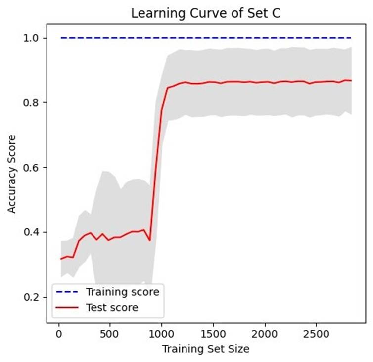
Nonetheless, to evaluate the classifier performance in terms of adding more data to the training set, we calculate learning curves using a size from 0 to 2500. We only made that computing from feature set C, since it has all types of parameters extracted. Figure 6 illustrates such a calculation.
Results and discussion
Under-sampling vs. oversampling
Since we have an unbalanced set of samples (78.9 % labeled as normal while 21.1 % as abnormal) it was necessary to implement a strategy to equalize the number of samples (rows of a data frame) for each class (i.e., to have the same number of samples labeled as normal or abnormal in each data frame). Most of the algorithms tackle this issue by randomly under-sampling the majority class; however, the main drawback of this technique is that potentially useful information contained in the ignored samples is neglected. We address the unbalanced classes problem by adopting two strategies: dropping entities of the majority class and oversampling of the minority class using SMOTE [70]. In heart sound classification, obtaining new recordings labeled as abnormal is not a simple task (there will always be more healthy people). SMOTE allows us to use the already acquired data and create "new" samples in the feature space as if it were possible to access more pathological heart sounds. Table 1, section I shows the classification scores when using the input features from data frames A-E and comparing the abovementioned balancing techniques. When oversampling is applied, the SP, ACC, and MCC all increased, while SE has decreased.
Table 1 Results from the PCG sounds classification after splitting the recordings in High Quality (HQR) and Low Quality (LQR) labels.
| Dataset | Balancing | SE | SP | ACC | MCC | Section |
|---|---|---|---|---|---|---|
| A | undersampling | 88.06 | 79.03 | 81.3 | 0.61 | I: HQR+LQR |
| B | 74.22 | 70.13 | 71.16 | 0.4 | ||
| C | 93.72 | 83.27 | 85.9 | 0.7 | ||
| D | 94.34 | 82 | 84.32 | 0.67 | ||
| E | 91.2 | 84.12 | 86.69 | 0.72 | ||
| A | oversampling | 71.07 | 94.07 | 88.28 | 0.68 | |
| B | 27.05 | 95.56 | 78.29 | 0.33 | ||
| C | 81.14 | 95.98 | 92.24 | 0.8 | ||
| D | 79.25 | 95.56 | 91.45 | 0.77 | ||
| E | 77.99 | 92.59 | 88.91 | 0.71 | ||
| A | undersampling | 76.99 | 82.47 | 81.39 | 0.52 | II: HQR |
| B | 65.49 | 72.51 | 71.13 | 0.32 | ||
| C | 87.61 | 82.25 | 83.3 | 0.6 | ||
| D | 61.95 | 92.86 | 86.78 | 0.57 | ||
| E | 87.61 | 82.25 | 83.3 | 0.6 | ||
| A | oversampling | 61.95 | 92.86 | 86.78 | 0.57 | |
| B | 28.32 | 95.89 | 82.61 | 0.34 | ||
| C | 76.11 | 93.94 | 90.43 | 0.7 | ||
| D | 78.76 | 94.16 | 91.13 | 0.72 | ||
| E | 78.76 | 91.13 | 88.7 | 0.66 | ||
| A | undersampling | 70 | 69.44 | 69.64 | 0.38 | III: LQR |
| B | 60 | 58.33 | 58.93 | 0.18 | ||
| C | 80 | 86.11 | 83.93 | 0.65 | ||
| D | 80 | 86.11 | 83.93 | 0.65 | ||
| E | 85 | 75 | 78.57 | 0.58 | ||
| A | oversampling | 55 | 75 | 67.86 | 0.3 | |
| B | 45 | 83.33 | 69.94 | 0.31 | ||
| C | 75 | 94.44 | 87.5 | 0.72 | ||
| D | 75 | 91.67 | 85.71 | 0.68 | ||
| E | 70 | 83.33 | 78.57 | 0.53 |
Effects of signal quality on performance
We analyzed the influence of signal quality in the algorithm performance. According to the noise condition labels mentioned in the low-quality recordings subsection, we evaluated the signals tagged as HQR (2,874) and LQR (279) separately. The oversampling and under-sampling balancing procedures were also considered. Table 1 also presents the results for the HQR and LQR, respectively. As expected, the scores are generally higher for the HQR compared to the highly noisy recordings. A more detailed analysis of the results is provided in the following section.
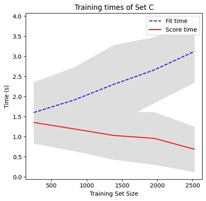
Training time evaluation
To assess the practicality and efficiency of the proposed schemes, we evaluated the training time of the algorithm. The results are shown in Figure 7; it can be seen that for 2,500 features in the training set, the computation time is below 4 seconds. This result is unsurprising since the amount of data is relatively small to use more sophisticated and computationally expensive classification algorithms, such as Deep Learning methods.
Feature selection
In order to keep the best parameters for classification and reduce overfitting and computational complexity in the proposed classification scheme, we implemented feature selection. There are features or variables in our data that are the most relevant, i.e., those that contribute the most to the output prediction. In the present work, we applied the Correlation Feature Selection (CFS) [76] and Information Gain (IG) methods [77] for this task. The reduced subset was constructed for the IG method, neglecting features that provided a null information gain (zero). Table 2 shows the feature selection results, presenting the number of features before and after. The CFS method works significantly better regarding dimensionality reduction, keeping only between 12 and 30 features, while IG varies between 50 and 116 attributes.
Table 2 Number of features in the datasets A-E originally produced, then number of reduced features after applying CFS and IG feature selection.
| Set | Original | Reduced CFS | Reduced IG |
|---|---|---|---|
| A | 90 | 22 | 66 |
| B | 90 | 20 | 65 |
| C | 146 | 30 | 116 |
| D | 131 | 22 | 101 |
| E | 56 | 12 | 50 |
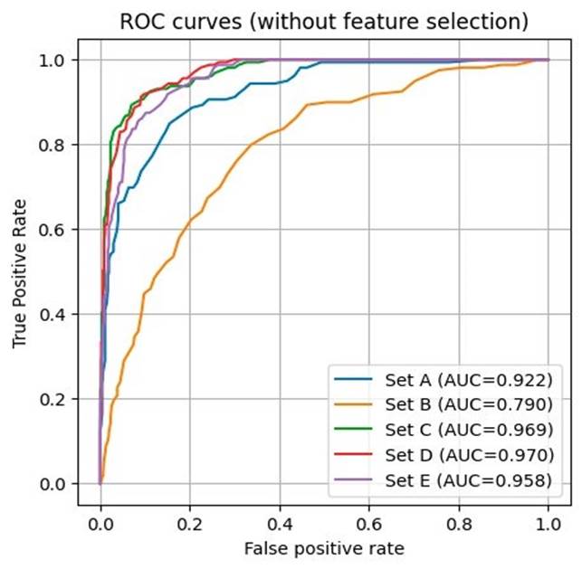
This section presents the classification performance evaluation when using feature selection by comparing the Receiver Operating Characteristics (ROC) curves and the calculation of the Area Under the Curve (AUC) for each feature set. Figure 8 shows the ROC curves for feature sets A-E. In this case, features set D exhibits the best performance since it has an AUC=0.97, the highest score obtained. However, set C is relatively close, showing AUC=0.969. This result suggests improving classification performance when adding MP and LPC parameters rather than only using MFCC or MP+LPC features. For cycle averaging, set B got the worst AUC score (0.79).
In another experiment, the ROC curves and AUC calculation was conducted when applying the CFS feature selection algorithm for each feature set, see Figure 9. There is an improvement in ACU scores since this metric increases for all feature sets. However, features set E now shows the best performance with an AUC=0.967. Feature sets C and D present a close AUC score of 0.961 and 0.967, respectively. On the other hand, although there is an increase from 0.76 to 0.867 for the AUC score of set B it is still the lowest obtained.
Figure 9 ROC curves and AUC for feature sets A-D after applying Correlation Feature Selection (CFS).
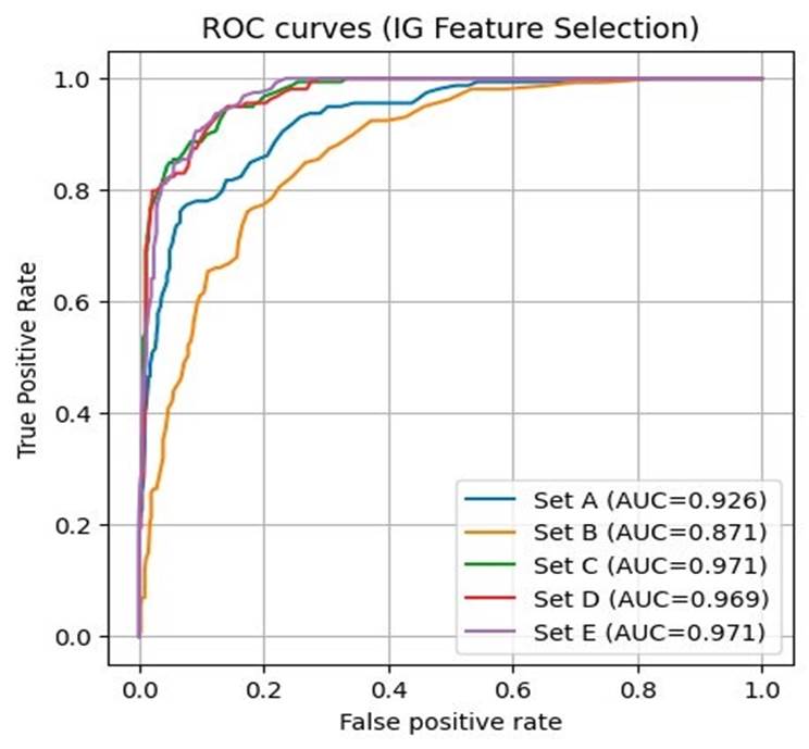
Finally, the same experiment was conducted but now using the features selected by the IG algorithm. Figure 10 shows the result. There is an improvement compared with results shown in Figure 9, when using CFS. However, feature sets C and D now show the best AUC score of 0.971, while in set D the AUC score is close (0.969). Set B is still presenting the worst ACU score (0.971).
Discussion
This work aimed to compare different feature extraction schemes based on spectral and sparse representations for the automated classification of heart sounds. A low-cost system with accurate automatic analysis could prove very useful in assisting early diagnosis and improving the prognosis of patients with cardiovascular diseases. The Physionet/CinC 2016 Challenge provides the research community with the largest open database of annotated heart sounds; the research presented in this paper employed this dataset. An algorithm performance comparison with a universally standardized database contributes to promoting advances in the field of automated heart sound analysis. Our key objective is to evaluate the performance of different feature extraction, balancing, and feature selection techniques that can be relevant for effectively detecting heart murmurs. After thoroughly examining various classification schemes, we selected the RF method for its simplicity and high performance [69]. The main reason to use MP+LPC as features stems from the heart sound reconstruction model we have previously proposed [71]. This sparse time-frequency model accurately represents the non-stationary behavior of the FHS and murmurs. The de facto standard feature for sound recognition are the MFCCs; they have been extensively used in PCG classification. In this work, we analyzed the classification performance for MP+LPC+MFCC. Comparing datasets A and B, all the output scores for set A are always higher than B's. In our tests, the feature averaging approach outperforms cardiac cycle averaging. We suppose that this fact results from the higher diversity produced when taking the mean value of the features rather than the direct calculation of the features from a single averaged cycle. The atomic decompositions in MP were performed using MPTK, the Matching Pursuit Toolkit [78].
Although dataset A displayed a good score (with best sensitivity SE=88.5 %) using undersampling, dataset E presents better results (best sensitivity SE=91.19 %). That is, classification based only on MFCC features outperforms the MP+LPC approach. Nevertheless, a combination of features improves the results as shown by the scores of datasets C and D. The merger of MP+LPC+MFCC ranked second in sensitivity SE=93.17 %, and dataset D (MP+MFCC) obtained the highest score (SE=94.34 %), both in case of using undersampling. In terms of feature selection, performance improved in terms of the AUC and ROC curve scores, the best obtained when applying the IG method. Feature sets D and E got an AUC=0.971, while set C obtained an AUC of 0.969, which is closer than the other sets. Although CFS produces a higher reduction in the number of features than the IG method and better results, the AUC scores are lower than when applying IG.
Conclusions
In this work, we analyzed the effects of detecting cardiac murmurs when applying the SMOTE oversampling and random-under sampling methods for class balancing. Classification algorithms work best in cases where the number of samples is balanced. The reason is that they are designed to maximize accuracy and reduce error. SMOTE creates new abnormal PCG synthetic instances using the existing (real) ones. Although highly desirable, increasing the number of abnormal PCG sounds is a challenging task.
For this reason, we opted to use SMOTE. However, it is essential to be aware that this procedure might increase the likelihood of overfitting since it replicates the minority class events. The obtained SE scores were higher for the case of undersampling. However, the remaining scores SP, ACC, and MCC were improved when applying SMOTE.
The selection of sparse and spectral features helps classify PCG recordings under a high noise level without using FHS segmentation. For the group of LQR samples, the algorithm reached a SE=85% in feature set E applying under-sampling. On the other hand, the SMOTE oversampling effects produced lower scores in LQR when applying cycle averaging (data frame B). The best results were achieved when using all LQR+HQR samples of the dataset.
Finally, we compared the effectiveness of our method when using information gain (IG) and correlation feature selection (CFS). The results after applying dimensionality reduction were slightly higher using less features than when using the whole set of attributes. The highest sensitivity obtained was SE=96.23 % when using under-sampling and feature set C for both CFS and IG, and for feature set D when using CFS. After inspecting the discarded features, we noticed that the phase of the time-frequency atoms selected by MP is not a relevant feature. This parameter was never chosen when using CFS, and it obtained a value of IG=0. This result is not surprising since, in general, the phase is considered a random variable uniformly distributed in the [-π,π] interval. In contrast, most of the MFCC were selected by both IG and CFS, in this case the first coefficients were ranked higher than the last. Regarding the other time-frequency atom parameters, the frequency, length, and position play a significant role in the classification. On the other hand, the amplitude has a low relevance. Only about a third of the coefficients were selected for the LPC without apparent order.
This research provides a complete assessment of feature selection methods for a classification algorithm to detect a pathological state from heart sounds. Different methods were evaluated, such as the balancing of samples, the comparison of MP+LPC vs. MFCC, and feature averaging vs. cycle time averaging as feature extraction methods. We also analyzed the effect of PCG signal quality and feature selection on classification performance. We selected the Random Forest technique algorithm to generate the classification model for PCG signals because the amount of data available is still small. Classical machine learning algorithms can often perform better than deep learning algorithms since they require a large amount of data for training. Nonetheless, classical machine learning algorithms are preferred when the interpretability of the model is essential since they are simpler and easier to understand [79].
The source code to reproduce the results of this paper can be downloaded free from; https://github.com/roilhi/ABMEPaperPCGClassif.git/.
Author contributions
R.F.I.H. conceptualized the project, performed data curation, contributed to the research and methodology, participated in the use of specialized software, and oversaw the project, obtained resources, and participated in the writing of the original draft of the manuscript. M.A.A.A. performed formal analyses, validated analyses, visualized results and supervised the development of the project, participated in the writing review and the editing of the manuscript. E.C.G.C. Obtained funding and economic resources, visualized results and supervised the development of the project, participated in the writing review and the editing of the manuscript. All authors reviewed and approved the final version of the manuscript.

