Introduction

Discharge estimation of hydrological basins based on rainfall-runoff analysis is a very frequent practice of Hydrology Engineering. But, also quite often, basin discharge measurements are not readily available for statistical analysis. This lack of information can be satisfactorily overcomed in most instances by using basin delineation and drainage morphometric analyses which provide resources for describing the hydrological behavior of a basin and are a prerequisite for runoff modeling (^{Magesh et al., 2011}; ^{Thomas et al., 2012}).

The conventional manually-made basin delineation method for large-area basins is a tedious and time-consuming job. As solution this situation, the advent of geographical information systems (GIS) tools have been developed to identify hydrologic basins using digital elevation models (DEM). This way, much of the traditional topographic map information can now be collected and processed digitally by using GIS-based data. The technique has been increasingly used to delineate river basins and to automatically extract morphometric parameters employed in hydrologic models. A well-known algorithm for automatic basin delineation is the Flow Direction Algorithm (^{O’Callaghan and Mark, 1984}), in which the flow direction follows the steepest gradient towards one out of eight neighbor pixels. These calculations are combined with accumulated flow in order to extract the drainage network and to delineate the basins. Flow accumulation, in its simplest form, is the quantity of up-slope cells that flow into a given cell. This technique is built upon the premise that surface flow follows the topography. Morphometric analyses have been widely used for characterizing basins. Some recent examples are: ^{Topaloglu, 2002}; ^{Moussa, 2003}; ^{Sreedevi et al., 2004}, ²⁰¹³; ^{Srinivasa Vittala et al., 2004}; ^{Mesa, 2006}; ^{Esper Angillieri, 2008}, ²⁰¹²; ^{Perucca and Esper Angillieri, 2011}. Recent studies using digital GIS-derived basin are: ^{Verstappen, 1983}; ^{Rinaldo et al., 1998}; ^{Farr and Kobrick, 2000}; ^{Macka, 2001}; ^{Grohmann, 2004}; ^{Gangalakunta, 2004}; ^{Godchild and Haining 2004}; ^{Grohmann et al., 2007}; ^{Korkalainen et al., 2007}; ^{Yu and Wei, 2008}; ^{Hlaing et al., 2008}; ^{Ozdemir and Bird, 2009}; ^{Panhalkar, 2014}. In addition, studies that compare delineation methods are: ^{Stanton, 2001}; ^{Baker et al., 2006}.

The current work aims at comparing the results from digital-manual delineation methods with those of automated delineations methods using GIS, in section of the Central Andean Cordillera of Argentina, while focusing on morphometric and peak discharge calculations. The method presented here is easy to reproduce and applicable to other mountain ranges of comparable topography and environment.

Study area

The study area comprises a sector of the Frontal Andean Cordillera, in the county of Iglesia, San Juan, at about 206 km NW from the city of San Juan, Argentina. The chosen area includes a section of National Road No. 150 up to the International Agua Negra pass between Argentina and Chile. It also includes the road access to the future international tunnel (Figure 1). The region presents a typical mountainous postglacial landscape, with open valleys and elevations ranging from 3,000 to 5,774 m a.s.l.. Despite the fact that current glacial activity has entered a retreating phase, the process has been considered an active relief modeling agent during past times. Erosive landforms such as cirques, glacial valleys arêtes and hanging valleys are common features. Some glacial accumulation landforms are longitudinal, basal and transversal moraines. Most representative periglacial landforms are rock glaciers, solifluction lobs, talus cones and asymmetrical valleys, with south-facing slopes being steeper than the north-facing ones.

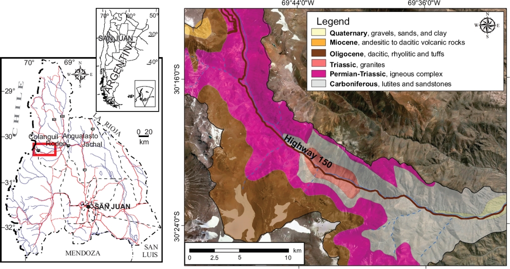
Figure 1 Location of the study area and lithological map. Image@2015CNES (SPOT 5) from Google Earth^TM. 

Material and methods

A topographic border for a given river basin determines the area in which all water volumes converge naturally towards a single given point. Based on the water divide line concept, the following procedures and tools were used to manually delineate basins on-screen. Fieldwork; high resolution satellite imageries (SPOT 5 with a 2.5 m spatial resolution, and IKONOS with a 4 m spatial resolution) from Google Earth^TM; digital topographic data (Aster GDEMV2) and GIS technology (ESRI's ArcGis 10.3).

In contrast, the same digital topographic data and GIS technology were used to extract basin contours automatically. The topographic basins limits can be calculated using the standard terrain analysis methods based on a DEM, which are implemented with most GIS software based on the algorithms of flow-direction and flow-accumulation functions. Flow directions were then calculated with the eight-direction (D8) flow model which assigns the flow direction from each grid cell to one of its eight adjacent cells, on the direction with the steepest downward slope. The D8 method was introduced by ^{O’Callaghan and Mark (1984)}.

Each basin was delimited by the position of its pour point, which is placed at or near the point of minimum elevation in the basin. The chosen pour point for each basin is shown in Figure 2. The topographic drainage divide of the basin is the line of highest topographic elevations that brings potential surface runoff to the basin’s pour point.

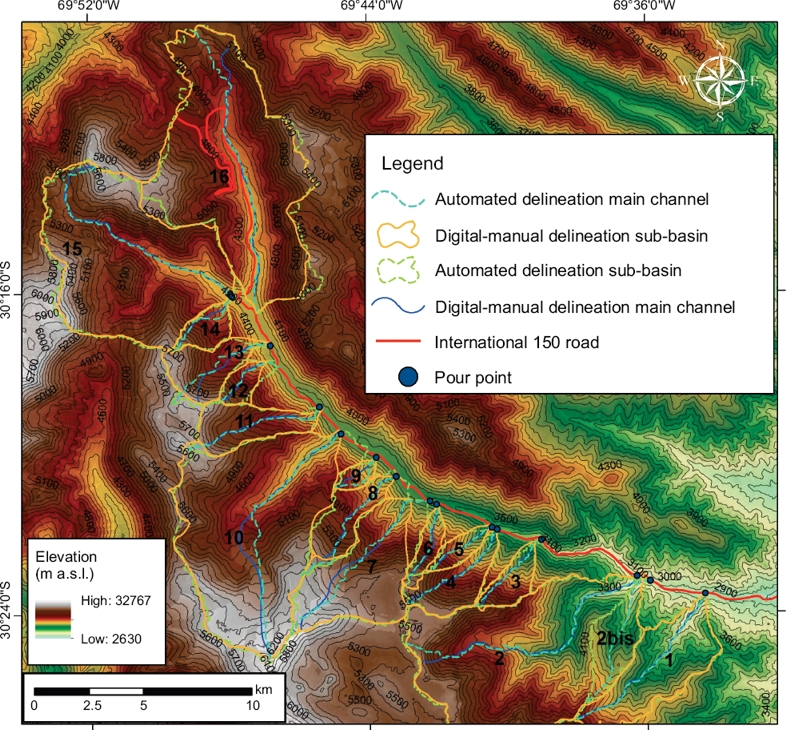
Figure 2 Digital-manual versus automated delineations of the sub-basins in the study area. Image@ digital topographic data (Aster GDEMV2). 

To evaluate the basin morphometry, various parameters were used: area (A), perimeter (P), length (L), mean width (W), maximum and minimum heights (H, h), main channel length (Mcl), form factor (^{Horton, 1932}), elongation ratio (^{Schumm, 1956}), sinuosity index (^{Schumm 1977}), basin relief (^{Hadley and Schumm 1961}), relief ratio (^{Schumm, 1956}) and Melton ratio (^{Melton, 1957}) were calculated (Table 1 and 2). The main channel length, or longest flow path, was identified by ^{Schumm (1956)} as the distance measured along the stream channel from source to outlet points. The distance can be measured using the available topographic data. In GIS software, the accumulated cost of travelling from the source grid cell (the outlet in this case) to each other grid cell in the raster dataset can be easily calculated. The source of the longest flow path can then be selected as the cell with the highest cost accumulation value. The distance to the outflow profile was calculated using the previously calculated flow direction grid (^{Zlatanović and Gavrić, 2013}).

Table 1 List of derived parameters, equations and references. Where: area (A), perimeter (P), length (L), mean width (W), maximum and minimum heights (H, h), main channel length (Mcl) and basin relief (Hr). 

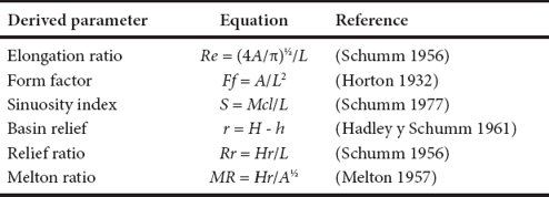
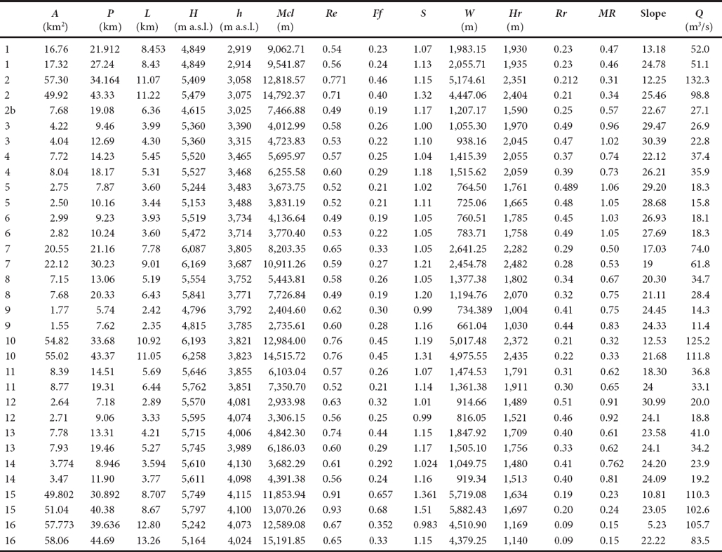
Table 2 Morphometric parameters and calculated peak discharge of basins. The values of digital-manual delineations basins are shown in gray shading. Where: area (A), perimeter (P), length (L), mean width (W), maximum and minimum heights (H, h), main channel length (Mcl), basin relief (Hr), Elongation ratio (Re), Form factor (Ff), Sinuosity index (S), Basin relief (r), Relief ratio (Rr), Melton ratio (MR). 

The Generalized Rational method (^{Rühle, 1966}) of estimating direct runoff from storm rainfall was chosen to estimate the peak discharge. This method relates peak discharge to contributing drainage area, rainfall intensity for a duration equal to a watershed response time (time of concentration by California Culvert Practice; ^{Department of Public Works, 1995}), and a coefficient that represents hydrologic abstractions and hydrograph attenuation. The basis of the method is the runoff equation, Equation (1):

(1)

were Q is peak discharge (m³/s), α is a coefficient that takes into account the influence of the lower intensity of rainfall on the area, β is a coefficient which takes into account the reduction of runoff by the soil characteristics (humidity, infiltration, etc.) of the drainage channel, A is the basin drainage area (ha), C is the runoff coefficient (dimensionless), R is the rainfall intensity i and K is a coefficient to standardize units.

Results and discussion

The manual digitization defined sixteen basins with varying areas (A), ranging from 1.78 to 57.77 km². In contrast, seventeen basins were delineated using the automatic computer method. When visually comparing both delineation methods (Figure 2), it is apparent that certain differences in line placement occurred. In some cases, however, e.g. basins 2, 6, 8 and 11, the computer-assisted delineations were more hydrologically correct than the manual ones. The comparison of the resulting morphometric characteristics and the calculated peak discharge is shown in Table 2 and Figure 3.

Figure 3 Comparison charts of principal morphometric parameters and peak discharge. 

The comparisons between manual and automated delineations were quantified (^{Stanton, 2001}) by: 1) comparing the total delineated area, 2) the percent “common area” of the manual delineated basins that was included in the computer delineated basins, 3) the percent area of the manual delineated basins that was underestimated by the computer method, and 4) the percent computer-delineated area extended beyond the manual drainage divide or the corresponding overestimate for the basins. Percent differences in area were calculated using absolute values of percent areas. The absolute value percent differences from computer-assisted and manually delineated basins areas averaged about 5.29 % and ranged from 0.50 to 13.83 %. The common area of the manual-delineated basins that was included in the computer-delineated basins averaged about 95.62 %. The area of the manual delineated sub-basins that was underestimated by the computer method averaged about 8.80 % and ranged from 4.28 to 12.88%. The computer-delineated area extended beyond the manual drainage divide or the corresponding overestimate of the basins averaged about 3.33 % and ranged from 0.35 to 7.10 %. These results indicate that the manual method is actually more prone to errors because it depends mainly on the experience and human judgment.

The shape factors, Re and Ff, show comparable values with both methods (Table 1). Elongation ratio (Re) and form factors (Ff) are important parameters in analyzing the basin shape. The estimated elongation ratio ranged from 0.48 to 0.93, which shows that the basins areas are characterized by high run off capacity along the stream flow path, a feature associated with high relief and steep slopes (^{Strahler, 1964}). The value of form factor was measured and ranged from 0.19 to 0.68. This indicates that the basins have more elongated shape in nature, with the characteristic of flatter peak flow for a longer duration. As such, elongated basins are highly vulnerable to flood flows than circular-shaped basin areas. Likewise, the basin relief (Hr) and relief ratio (Rr) show similar values by both methods, and these parameters indicate the intensity of the erosion process operating on the slope of the basins, low infiltration, and high runoff conditions.

The basin relief (Table, 1) is also closely matched for both methods, showing that the overall vertical precision of the DEM is satisfactory for spatial analysis at this scale. The results comparisons for the main channel length showed that the Mcl is generally slightly longer for all basins when using the automatic extraction from DEM, with 17.35% on average. Nonetheless, these differences do not greatly affect further calculations, such as sinuosity (Table 2 and Figure 3). In general, the Melton ratio (MR) values are > 0.3, which imply a moderate probability of experiencing frequent flooding with low material content. Nevertheless, these statements can be relatively interpreted, because it will depend on the dimensions or extent of the storm as well as its duration and intensity. On the other hand, the probability for hydrograms of floods with pronounced peaks of short duration occurrence is high, considering the high relief and recent events. Similar results were obtained and reported in ^{Esper Angillieri and Perucca (2014a}, ^2014b).

The average catchment's slope showed marked differences when the two methods were compared (Figure 3). This can be attributed to the different methodologies applied. When calculating the slope manually using topographic maps, the area between two neighboring elevation contours is treated with uniform slope, whereas when calculating the slope using a DEM, it is calculated for every grid cell, thus taking into account the spatial variability of the slope over the catchment area. This implies that the slopes calculated through the computer-assisted method are much highly accurate than those calculated with the manual method. Similar results were obtained by ^{Zlatanović and Gavrić (2013)}.

In examining the resulting peak discharges (Table 2 and Figure 3), it can be noted that Flow rates obtained by automated methods proved to be slightly smaller than those manually obtained, although the difference was less than 6.1% on average. Furthermore, these figures point to a high probability for serious flood hazard, with peak discharges greater than 100 m³/s.

It is appropriate to take into account that the automatic extraction of basins was conducted using DEM of 30 m resolution, which subsequently restricts the accuracy of the estimated drainage areas. In hydrology, the drainage area of a basin is needed as the basis for a large number of calculations. Thus, uncertainties in the basin area will definitely lead to uncertainties of the same order into the rest of calculations. Therefore, it turns an essential duty to determine the basin area as precisely as possible. The smaller the cell size, the greater the resolution. Therefore, smaller basins require a smaller cell size to accurately represent the basin area.

Finally, the manual on-screen digitalized method is slower than the raster process, and is ultimately based on human interpretation of satellite imageries and topographic contour maps.

Conclusions

The hydrologic unit delineation study of basins in the study area in Northwestern Argentina was aimed at comparing the computer delineation method with the manual traditional method for delineating basins. In performing automatic delineation, flow directions were computed, and a flow accumulation grid was generated. Moreover, through field observations and high resolution satellite imagery interpretation, along with the help of some tools of GIS environment, the main morphometric parameters for the two methods were calculated and contrasted.

The computed morphometric characteristics of basins in the study area revealed that the basins are elongated, with high relief and steep slope. The Melton ratio (MR) indicates a great susceptibility of the basin to the occurrence of stream flows. The values obtained from the peak discharge calculations point to a high occurrence probability for serious flood hazard, with peak discharges greater than 100 m³/s.

Delineating basins and measuring morphometric parameters by the traditional manual method require time, precise workmanship and judgments by specialists. In contrast, for the same analysis, the automated techniques reduce the computation to just few minutes. However, it should be kept in mind that the automated procedure is not completely foolproof and some degree of judgment and subjectivity may be required as well.

Finally, the results presented in this paper could be included as a tool when planning, designing, and managing the roads through areas featuring similar conditions as those of the present work.