


 nueva página del texto (beta)
 Inglés (pdf)
 Artículo en XML
 Referencias del artículo
 Enviar artículo por email
 Citado por SciELO
  Similares en
SciELO
Similares en
SciELO 
 Permalink
1 Introduction
At present, Intelligent Transportation Systems (ITS) is an advanced application combining engineering transport, communication technologies and geographical information systems. These systems [15] play a significant part in minimizing the risk of accidents, the traffic jams and pollution. Also, ITS improve the transport efficiency, safety and security of passengers. They are used in various domains such as railways, avionics and automotive technology. At different steps, several applications need to use sorting algorithms such as decision support systems, path planning [6], scheduling and so on.
However, the complexity and the targeted execution platform(s) are the main performance criteria for sorting algorithms. Different platforms such as CPU (single or multi-core), GPU (Graphics Processing Unit), FPGA (Field Programmable Gate Array) [14] and heterogeneous architectures can be used.
Firstly, the FPGA is the most preferable platform for implementing the sorting process. Thus, industry uses frequently FPGAs for many real-time applications improve performance in terms of execution time and energy consumption [4,5]. On the other hand, using an FPGA board allows to build complex applications which have a high performance. These applications are being made by receiving a large number of available programmable fabrics. They provide an implementation of massively-parallel architectures [5]. The increase in the complexity of the applications has led to high-level design methodologies[10]. Hence, High-Level Synthesis (HLS) tools have been developed to improve the productivity of FPGA-based designs.
However, the first generation of HLS has failed to meet hardware designers' expectations; some reasons have facilated researchers to continue producing powerful hardware devices. Among these reasons, we quote the sharp increase of silicon capability; recent conceptions tend to employ heterogeneous Systems on Chips (SoCs) and accelerators. The use of behavioral designs in place of Register-Transfer-Level (RTL) designs allows improving design productivity, reducing the time-to-market constraints, detaching the algorithm from architecture to provide a wide exploration for implementing solutions [11]. From a high-level programming language (C / C ++), Xilinx created the vivado HLS [34] tool to generate hardware accelerators.
The sorting algorithm is an important process for several real-time embedded applications. There are many sorting algorithms [17] in the literature such as BubbleSort, InsertionSort and SelectionSort which are simple to develop and to realize, but they have a weak performance (time complexity is O(n 2)). Several researchers have used MergeSort, HeapSort and QuickSort with O(nlog(n)) time complexity to resolve the restricted performance of these algorithms [17]. On the one hand, HeapSort starts with the construction of a heap for the data group. Hence, it is essential to remove the greatest element and to put it at the end of the partially-sorted table. Moreover, QuickSort is very efficient in the partition phase for dividing the table into two. However, the selection of the value of the pivot is an important issue. On the other hand, MergeSort gives a comparison of each element index, chooses the smallest element, puts them in an array and merges two sorted arrays.
Furthermore, other sorting algorithms are improving the previous one. For example, ShellSort is an enhancement of the insertion sort of algorithm. It divides the list into a minimum number of sub-lists which are sorted with the insertion sort algorithm. Hybrid sorting algorithms emerged as a mixture between several sorting algorithms. For example, Timsort combines MergeSort and InsertionSort. These algorithms choose the InsertionSort if the number of elements is lower than an optimal parameter (OP) which depends on the target architecture and the sorting implementation; otherwise, MergeSort is considered with integrating some other steps to improve the execution time.
The main goal of our work is to create a new simulator which simulates the behavior of elements / components related to intelligent transportation systems; In [2], the authors implemented an execution model for a future test bench and simulation. However, they propose a new hardware and software execution support for the next generation of test and simulation system in the field of avionics. In [33], the authors developed an efficient algorithm for helicopter path planning. They proposed different scheduling methods for the optimization of the process on a real time high performance heterogeneous architecture CPU/FPGA. The authors in [25] presented a new method of 3D path design using the concept of "Dubins gliding symmetry conjecture". This method has been integrated in a real-time decisional system to solve the security problem.
In our research group, several researchers proposed a new adaptive approach for 2D path planning according to the density of obstacle in a static environment. They improved this approach into a new method of 3D path planning with multi-criteria optimizing. The main objective of this work is to propose a different optimized hardware accelerated version of sorting algorithms (BubbleSort, InsertionSort, SelectionSort, HeapSort, ShellSort, QuickSort, TimSort and MergeSort) from High-Level descriptions in avionic applications. We use several optimization steps to obtain an efficient hardware implementation in two different cases: software and hardware for different vectors and permutations.
The paper is structured as follows: Section II presents several studies of different sorting algorithms using different platforms (CPU, GPU and FPGA). Section III shows a design flow of our application. Section IV gives an overview of sorting algorithms. Section V describes our architecture and a variety of optimizations of hardware implementation. Section VI shows experimental results. We conclude in Section VII.
2 Background and Related Work
Sorting is a common process and it is considered as one of the well-known problems in the computational world. To achieve this, several algorithms are available in different research works. They can be organized in various ways:
- Depending on the algorithm time complexity, Table I presents three different cases (best, average and worst) of the complexity for several sorting algorithms. We can mention that QuickSort, HeapSort, MergeSort, timSort have a best complexity of O(nlog(n)) in average case. By contrast, the worst case performance for the four algorithms is O(n 2) obtained by QuickSort. A simple pretest makes all algorithms in the best case to O(n) complexity.
- Each target implementation platform, such as CPUs, GPUs, FPGAs and the hybrid platform, has a specific advantage: FpGa is the best platform in terms of power consumption while CPU is considered as a simple platform for programmability. GPU appears as a medium solution.
The authors in [9] used MergeSort to sort up to 256M elements on a single Intel Q9550 quadcore processor with 4GB RAM for single thread or multi-thread programs, whereas the authors in [29] considered the hybrid platform SRC6 (CPU Pentium 4+FPGA virtex2) for implementing different sorting algorithms (RadixSort, QuickSort, HeapSort, Odd-EvenSort, MergeSort, BitonicSort) using 1000000 elements encoded in 64 bits [17].
- According to the number of elements to be sorted, we choose the corresponding sorting algorithms. For example, if the number of elements is small, then InsertionSort is selected, otherwise; MergeSort is recommended.
Table 1 Complexity of the sorting algorithms
| Best | Average | Worst | |
|---|---|---|---|
| BubbleSort | O(n) | O(n 2) | O(n 2) |
| InsertionSort | O(n) | O(n 2) | O(n 2) |
| SelectionSort | O(n 2) | O(n 2) | O(n 2) |
| HeapSort | O(n log(n)) | O(n log(n)) | O(n log(n)) |
| ShellSort | O(n log(n)) | O(n log(n)2) | O(n log(n)2) |
| QuickSort | O(n log(n)) | O(n log(n)) | O(n 2) |
| MergeSort | O(n log(n)) | O(n log(n)) | O(n log(n)) |
| TimSort | O(n) | O(n log(n)) | O(n log(n)) |
Zurek et al. [35] proposed two different hardware implementation algorithms: the quick-merge parallel and the hybrid algorithm (parallel bitonic algorithm on the GPU + sequence MergeSort on CPU) using a framework openMP and CUDA. They compared two new implementations with a different number of elements. The obtained result shows that multicore sorting algorithms are the best scalable and the most efficient. The GPU sorting algorithms, compared to a single core, are up to four times faster than the optimized quick sort algorithm. The implemented hybrid algorithm (executed partially on CPU and GPU) is more efficient than algorithms only run on the GPU (despite transfer delays) but a little slower than the most efficient, quick-merge parallel CPU algorithm. They showed that the hybrid algorithm is slower than the most efficient quick-merge parallel CPU algorithm.
Abiramiet al. [1] presented an efficient hardware implementation of the MergeSort algorithm with Designing Digital Circuits. They measured the efficiency, reliability and complexity of the MergeSort algorithm with a digital circuit. Abirami used only 4 input and compared the efficiency of the MergeSort to the bubble sort and the selection sort algorithms. The disadvantage of this work is using only MergeSort algorithm in FPGA.
Pasetto et al. [26] presented several parallel implementations of five sorting algorithms (MapSort, MergeSort, Tsigas-Zhang's Parallel QuickSort, Alternative QuickSort and STLSort) using an important number of elements. They calculated the performance of this algorithm using two different techniques (direct sorting and key/pointer sorting) and two machines: Westmere (Intel Xeon 5670, frequency: 2.93 GHz and 24 GB of memory) containing 6 cores i7 and Nehalem (Intel Xeon 5550, 2.67 GHz, 6 GB of memory) integrating 4 cores i7. After that, they compared the several algorithms in terms of CPU affinity, throughput, microarchitecture analysis and scalability.
Based on the obtained results, the authors recommended MergeSort and MapSort when memory is not an issue. Both of these algorithms are advised if the number of elements is up to 100000, as they need an intermediate array size. Danelutto et al. [12] presented an implementation of the pattern using the openMP, the Intel TBB framework and the Fastflow parallel programming running on multicore platforms. They proposed a high-level tool for the fast prototyping of parallel Divide and Conquer algorithms. The obtained results show that the prototype parallel algorithms allow a reduction of the time and also need a minimum of programming effort compared to hand-made parallelization.
Jan et al. [19] presented a new parallel algorithm named the min-max butterfly network, for searching a minimum and maximum in an important number of elements collections. They presented a comparative analysis of the new parallel algorithm and three parallel sorting algorithms (odd even sort, bitonic sort and rank sort) in terms of sorting rate, sorting time and speed running on the CPU and GPU platforms. The obtained results show that the new algorithm has a better performance than the three others algorithms.
Grozea et al. [25] allowed to accelerate existing comparison algorithms (MergeSort, Bitonic Sort, parallel Insertion Sort) (see, e.g. [22,28] for details) to work at a typical speed of an Ethernet link of 1 Gbit/s by using parallel architectures (FPGAs, multi-core CPUs machines and GPUs). The obtained results show that the FPGA platform is the most flexible, but it is less accessible. Beside that GPU is very powerful but it is less flexible, difficult to debug and requiring data transfers to increase the latency. Sometimes, the CPU is perhaps too slow in spite of the multiple cores and the multiple CPUs, but it is the easiest to use.
Konstantinos et al [16] proposed an efficient hardware implementation for three algorithms based on virtex 7 FPGAs of image and video processing using high level synthesis tools to improve the performance. They focused only in the MergeSort algorithm for calculating the Kendall Correlation Coefficient. The obtained results show that the hardware implementation is 5.6x better than the software implementation. Janarbek et al. [16] proposed a new framework which provides ten basic sorting algorithms for different criteria (speed, area, power…) with the ability to produce hybrid sorting architectures. The obtained results show that these algorithms had the same performance as the existing RTL implementation if the number of elements is lower than 16K elements whereas they overperformed it for large arrays (16K-130K). We are not in this context because the avionic applications need to sort at most 4096 elements issuing from previous calculation blocs.
Chen et al. [8] proposed a methodology for the hardware implementation of the Bitonic sorting network on FPGA by optimizing energy and memory efficiency, latency and throughput generate high performance designs. They proposed a streaming permutation network (SPN) by "folding" the classic Clos network. They explained than the SPN is programmable to achieve all the interconnection patterns in the bitonic sorting network. The re-use of SPN causes a low-cost design for sorting using the smallest number of resources.
Koch et al. [21] proposed an implementation of a highly scalable sorter after a careful analysis of the existing sorting architectures to enhance performance on the processor CPU and GPUs. Moreover, they showed the use of a partial run time reconfiguration for improving the resource utilization and the processing rate…
Purnomo et al. [27] presented an efficient hardware implementation of the Bubble sort algorithm. The implementation was taken on a serial and parallel approach. They compared the serial and the parallel bubble sort in terms of memory, execution time and utility, which comprises slices and LUTs. The experimental results show that the serial bubble sort used less memory and resource than the parallel bubble sort. In contrast, the parallel bubble sort is faster than the serial bubble sort using an FPGA platform.
Other researchers works on high-speed parallel schemes for data sorting on FPGA are presented in [13,4]. Parallel sorting which was conducted by Sogabe [32] and Martinez [24]. Finally the comparison study of many sorting algorithms covering parallel MergeSort, parallel counting sort, and parallel bubble sort on FPGA is an important step [7].
The obtained results in a certain amount of works which aim to parallelize the sorting algorithms on several architectures (CPU, GPU and FPGA) show that the speedup is proportional to the number of processors. These researches show that the hardware implementation on FPGA give a better performance in terms of time and energy. In this case, we can parallelize to the maximum but we do not reach the values of speedup because the HLS tool could not extract enough parallelization since we need only a small number of elements to be sorted.
Hence, the HLS tool improves hardware accelerator productivity while reducing the time of design. Also, the major advantage of HLS is the quick exploration of the design space to find the optimal solution. HLS Optimization Guidelines Produce Hardware IP that verifies Surface and Performance Tradeoff. We notice that there are several algorithms not used for FPGA. To this end, we choose in this work the FPGA platform and the HLS tool to improve performance and to select the best sortng algorithm.
We proposed in our previous work [20] an efficient hardware implementation of MergeSort and TimSort from high-level descriptions using the heterogeneous architecture CPU/FPGA. These algorithms are considered as part of a real-time decision support system for avionic applications. We have compared the performance of two algorithms in terms of execution time and resource utilization. The obtained results show that TimSort is faster than MergeSort when using an optimized hardware implementation.
In this paper, we proposed an improvement of the previous work based on the permutation generator proposed by Lehmer to generate the different vectors and permutations as input parameter. we compared the 8 sorting algorithms (BubbleSort, InsertionSort, SelectionSort, ShellSort, QuickSort, HeapSort, MergeSort and TimSort) implemented on FPGA using 32 and 64 bit encoded data. Table 2 presented the comparative analysis approaches of the discussed studies.
Table 2 Different context analysis approaches
| Approach | Algorithms | Parallelization | Platforms | Avionic application | High Level tool | ||||
|---|---|---|---|---|---|---|---|---|---|
| Name | Complexity | High performance | CPU | GPU | FPGA | ||||
| MergeSort | O(n log(n)) | ||||||||
| Grozea et al [10] | Bitonic sort | O(n log(n)ˆ2) | Yes | Yes | Yes | Yes | Yes | No | No |
| Parallel InsertionSort | O (nˆ2) | ||||||||
| Chhugani et al [11] | MergeSort | O(n log (n)) | Yes | Yes | Yes | No | No | No | No |
| Satish et al [12] | RadixSort | O(nK) | Yes | Yes | No | Yes | No | No | No |
| MergeSort | O(n log(n)) | ||||||||
| Zurek et al [13] | Parallel quick merge Hybrid algorithm |
- | Yes | Yes | Yes | Yes | No | No | Yes |
| Abirami et al[14] | MergeSort | O(n log (n)) | Yes | Yes | No | No | Yes | No | No |
| MapSort | O(n/P(log(n)) | ||||||||
| MergeSort | O(n log(n)) | ||||||||
| Pasetto et al [15] | Tsigas-Zhangs | O(n log(n)) | Yes | Yes | Yes | No | No | No | No |
| Alternative QuickSort | O(n log(n)) | ||||||||
| STLSort | - | ||||||||
| Danelutto et al [16] | Divide and conquer | O(n log(n)) | Yes | Yes | Yes | No | No | No | Yes |
| Jan et al [17] | min-max butterfly | - | Yes | Yes | Yes | Yes | No | No | No |
| Konstantinos et al [20] | MergeSort | O(n log(n)) | Yes | Yes | Yes | No | Yes | No | Yes |
| Chen et al [21] | BitonicSort | O(n log(n)ˆ2) | Yes | Yes | No | No | Yes | No | No |
| Koch et al [22] | Highly scalable sorter | - | Yes | Yes | Yes | Yes | No | No | No |
| Purnomo et al [23] | BubbleSort | O(nˆ2) | Yes | Yes | No | No | FPGA | No | No |
| MergeSort | O(n log(n)) | ||||||||
| [24 25 26 27 28] | Parallel CountingSort | O(n+k) | Yes | Yes | No | No | Yes | No | No |
| Parallel BubbleSort | O(nˆ2) | ||||||||
| Previous work [29] | MergeSort | O(n log(n)) | Yes | Yes | Yes | No | Yes | Yes | Yes |
| TimSort | O(n log(n)) | ||||||||
| BubbleSort | O(nˆ2) | ||||||||
| InsertionSort | O(nˆ2) | ||||||||
| SelectionSort | O(nˆ2) | ||||||||
| Our work | QuickSort | O(n log(n)) | Yes | Yes | Yes | No | Yes | Yes | Yes |
| HeapSort | O(n log(n)) | ||||||||
| MergeSort | O(n log(n)) | ||||||||
| ShellSort | O(n(log(n)ˆ2)) | ||||||||
| TimSort | O(n log(n)) | ||||||||
3 Design Flow
To accelerate the different applications (real time decision system, 3D path planning) , Figure 1 presents the general structure of the organization for design. Firstly, we have a set of tasks programmed in C/C++ and to be executed on a heterogeneous platform CPU/FPGA. After that, we optimize the application via High Level Synthesis(HLS) tool optimization directives for an efficient hardware implementation. In addition, we optimize these algorithms by an another method that runs in parallel the same function with different input. Next, the optimized program will be divided into software and hardware tasks using the different metaheuristic or a Modified HEFT (Heterogeneous Earliest-Finish Time) (MHEFT) while respecting application constraints and resource availability. This step is proposed in [33]. The hardware task will be generated using the Vivado HLS tool from C/C++. Finally, the software and the hardware tasks will communicate with bus to run them on the FPGA board. This communication is done with ISE or vivado tools to obtain an efficient result implementation.

4 Overview of Sorting Algorithms
4.1 BubbleSort
Bubble sort [31,24] is a simple and well-known algorithm in the computational world.
However, it is inefficient for sorting a large number of elements because its complexity is very important O(n 2) in the average and the worst case. Bubble sort is divided into four steps. Firstly, bubble sort is the high level, which allows sorting all input. The second step is to swap two inputs if tab[j]>tab[j+1] is satisfied. Subsequently, the comparator step makes it possible to compare two inputs. Finally, an adder is used to subtract two inputs to define the larger number in the comparator component. These different steps are repeated until you sorted array is obtained (Figure 2).

4.2 SelectionSort
The selection sorting algorithm [18] is a simple algorithm for analysis, compared to other algorithms. Therefore, it is a very easy sorting algorithm to understand and it is very useful when dealing with a small number of elements. However, it is inefficient for sorting a large number of elements because its complexity is O(n 2) where n is the number of elements in the table. This algorithm is called SelectionSort because it works by selecting a minimum of elements in each step of the sort. The important role of selection sort is to fix the minimum value at index 0. It searches for the minimum element in the list and switches the value at the medium position. After that, it is necessary to increment the minimum index and repeat until the sorted array is obtained (Figure 3).

4.3 InsertionSort
InsertionSort [31] is another simple algorithm used for sorting a small number of elements as shown in Figure 4. Nevertheless, it has a better performance than BubbleSort and SelectionSort. InsertionSort is less efficient when sorting an important number of elements, which requires a more advanced algorithm such as QuickSort, HeapSort, and MergeSort because its complexity is very important O(n 2) in the average and the worst case. The InsertionSort algorithm is used to integrate a new element in each iteration and to compare the values of elements in the list. If the value of an element is less than the current value of that element then a switch is performed. Repeat this step until n-1 item.

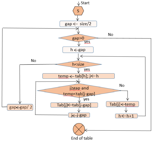
4.4 ShellSort
ShellSort [30] is a very efficient sorting algorithm for an average number of elements and it is an improvement of the InsertionSort algorithm as it allows to switch the elements positioned further. The average-case and worst-case complexities of this algorithm are of O(n(1og(n)2)). The principle role of this algorithm is to compute the value of h and divides the list into smaller sub-lists of equal h intervals. After that, it sort each sub-list that contains a large number of elements using InsertionSort. Finally, repeat this step until a sorted list is obtained. ShellSort is not widely used in the literature.
4.5 QuickSort
Quicksort [23] is based on a partitioning operation: Firstly, this algorithm divides a large array into two short sub-arrays: the lower elements and the higher elements. It is divided into different steps:
Select an element from array, named pivot.
Partitioning: move all smaller elements'values before the pivot, and move all bigger'elements values after it. After this partitioning, the pivot is in its final position, called partition operation.
Repeat recursively the different steps for two sub-arrays with smaller and greater values of elements.
Therefore, it is a divide and conquer algorithm. Quicksort is faster in practice than other algorithms such as BubbleSort or Insertion Sort because its complexity is O(n log n). However, the implementation of QuickSort is not stable and it is a complex sort, but it is among the fastest sorting algorithms in practice.
The most complex problem in QuickSort is selecting a good pivot element. Indeed, if at each step QuickSort selects the median as the pivot it will obtain a complexity of O(n log n), but a bad selection of pivots can always lead to poor performance (O(n 2) time complexity), cf. Figure 6.

4.6 HeapSort
HeapSort [3] is based on the same principle as SelectionSort, since it searches for the maximum element in the list and places this element at the end. This procedure is repeated for the remaining elements. This algorithm is a better sorting algorithm being in place because its complexity is O(n log(n)). In addition, this algorithm is divided into two basic steps:
- Creating a Heap data structure (Max-Heap or Min-Heap) with the first element of the heap, which is the greatest or the smallest (depending upon Max-Heap or Min-Heap)
- Repeating this step using the remaining elements to select again the first element of the heap and to place this element at the end of the table until you get a sorted array. Heapsort is too fast and it is not stable sorting algorithm. It is very widely used to sort a large number of elements.

4.7 MergeSort
In 1945, MergeSort [20] was established by John von Neumann. The implementation of this algorithm retains the order of input to output. Therefore, this algorithm is an efficient and stable algorithm. It is based on the famous divide and conquer paradigm. The necessary steps of this algorithm are : 1- Divide array into two sub-arrays, 2- Sort these two arrays recursively 3- Merge the two sorted arrays to obtain the result. It is a better algorithm than the HeapSort, QuickSort, ShellSort and TimSort algorithms because its complexity in the average case and the worst case is O(n log(n)) but its is O(n log(n)) in the best case as shown in Figure 8.

4.8 TimSort
TimSort [20] is based on MergeSort and Insertion-Sort algorithms. The principle role of this algorithm is to switch between these two algorithms. This step depends on the value of the optimal parameter (OP) which is fixed to 64 for the architecture of the processor Intel i7. The execution time is almost equal for parallel architectures when we change the value of parameter OP. Therefore, we consider in this work the value of OP is 64 because several research use this standardized value. However, we could follow two different ways by mean of the size of elements to be sorted: If the size of the array is greater or equal than 64 elements, then MergeSort will be considered; otherwise, InsertionSort is selected in the sorting step as shown in Figure 9.

5 Optimized Hardware Implementation
In this section, we will present the different optimizations applied to the sorting algorithms defined in the previous section using HLS directives with the size of data 64 bits. Then, we will explain our execution architecture. Finally, we will propose several input data using the Lehmer method to take a final decision.
5.1 Optimization of Sorting Algorithms
In order to have an efficient hardware implementation, we applied the following optimization steps to the C code for each sorting algorithm:
- Loop unrolling: The elements of the table are stored in BRAM memory, which are described by dual physical ports. The dual ports could be configured as dual write ports, dual read ports or one port for each operation. We profit from this optimization by unrolling the loops in the design by factor=2. For example, only writing elements are executed in the loop. Hence, the two ports for an array could be configured as writing ports and consequently we could unroll the loop by factor=2.
- Loop iterations are pipelined in order to reduce the execution time. Loop iterations are pipelined in our design with only one clock cycle difference in-between by applying loop pipelining with Interval iteration (II)=1. To satisfy this condition, the tool will plan loop execution.
- Input/output Interface: Input/output ports are configured to exploit the AXI-Stream protocol for data transfer with minimum communication signals (DATA, VALID and READY). Also, the AXI-Lite protocol is employed for design configuration purposes; for example, to determine the system's current state (start, ready, busy).
5.2 Hardware Architecture
Today, the heterogeneous architecture presents a lot of pledge for high performance extraction by combining the reconfigurable hardware accelerator FPGA with the classic architecture. The use of this architecture causes a significant improvement in performance and energy efficiency. In the literature, different heterogeneous architectures such as Intel HARP, Microsoft Catapult and Xilinx Zynq are used.this architecture promises a massive parallelism for proceeding improvement in hardware acceleration of the FPGA technology. In fact, the FPGA technology can offer a better performance (power consumption, time…), up to 10 times compared to the CPU. We use in this work a Xilinx Zynq board which has two different modes of communication: AXI4-Lite and AXI4-Stream.
In this case, we choose the AXI4-Stream protocol in this paper because it is one of the AMBA protocols designed to carry streams of Arbitrary width data of 32/64 bit size in the hardware. These data are generally represented as vector data on the software side that can be transferred 4 bytes per cycle. On one side, the AXI4-Stream is designed for high-speed streaming data. This mode of transfer supports unlimited data burst sizes and provides point-to-point streaming data without using any addresses. However, it is necessary to fix a starting address to begin a transaction between the processor and HW IP. Typically, the AXI4-Stream interface is used with a controller DMA (Direct Memory Access) to transfer much of the data from the processor to the FPGA as presented in Figure 10. In this case, An interrupt signal is invoked when the first packet of data is transferred, for the associated channel to initialize a new transfer. On the one hand, we consider that the scatter-gather engine option is disabled on the AXI DMA interface.

Figure 10 shows how the HLS IP (HLS is sorting) is connected to the design. The input data are stored in the memory of the processing element (DDR Memory). They are transferred from the processing system (ZYNQ) to the HLS core (HLS Sorting Algorithm) through AXI-DMA communication. After the data are sorted, the result is written back through the reverse path.
5.3 Choice of the Input Data
In this part, we propose different input data, which are stored in several file systems. Firstly, we present the management of files on an SD card (Secure Digital Memory Card) while retaining a strong portability and practicality from the FPGA. SD cards are not easily eresable enforceable with FPGAs and are widely used the portable storage medium. Nowadays, several studies show that using the SD card controller with FPGA play an important role in different domains. They are based on the use of an API interface (Application Programming Interface), AHB bus (Advanced High performance Bus), etc. They are dedicated to the realization of an ultra-high-speed communication between the SD card and upper systems. All the communication is synchronous to a clock provided by the host (FPGA). The file system design and implementation of an SD card provides three major means of innovation:
- The integration and combination of the SD card controller and the file system, gives a system which is highly incorporated and convenient.
- The utilization of file management makes processing easier. In addition, it improves the overall efficiency of the systems.
- The digital design provides a high performance and it allows a better portability since it is independent of the platform.
In this paper, we implemented the different algorithms using many data encoded in 8 bytes,which is another solution for optimizing the performance. Thus, several studies in computer science on sorting algorithms use the notion of permutations as input.
5.3.1 Permutation
Firstly, permutation is used with different combinatory optimization problems especially in the field of mathematics. Generally, a permutation is an arrangement of a set of n objects 1,2,3,,n into a specific order and each element occurs just only once. For example, there are six permutations of the set 1,2,3, namely (1,2,3), (1,3,2), (2,1,3), (2,3,1), (3,1,2), and (3,2,1). So, the number of permutations depends only on the n objects. In this case, there are exactly n! permutations. Secondly, a permutation π is a bijective function from a set 1,2,...,n to itself (i.e., each element i of a set S has a unique image j in S and appears exactly once as image value). We also considered that pos π (i) is the position of the element i in the permutation π; π(i); is the element at position i in π and S n is a set of all the possibilities of permutation of size n. Among the many methods used to treat the problem of generating permutations, the Lehmer method is used in this paper.
6 Experimental Results
In this section, we present our results of execution time and resource utilization for sorting algorithms on Software and Hardware architecture. We compare our results for different cases: Software and optimized hardware for several permutations and vectors. A set of R=50 replications is obtained for each case and permutations/vectors. The array size ranges from 8 to 4096 integers encoded in 4 and 8 bytes. As previously mentioned, we limited the size to 4096 elements because the best sorting algorithm is mainly used for real-time decision support systems for avionic applications. In this case, it sorted at most 4096 actions issuing from the previous calculation blocks.
We developed our hardware implementation using a Zedboard platform. The hardware architecture was synthesized using the vivado suite 2015.4 with default synthesis/implementation strategies. Firstly, we compared the execution time between several sorting algorithms on a software architecture (processor Intel core i3-350M)). The frequency of this processor is 1.33 GHz. Table 3 reports the average execution time of each algorithm for different sizes of arrays ranging from 8 to 4096 elements with 50 replications (R=50).
Table 3 Execution time of different algorithms
| BubbleSort (US) | InsertionSort (US) | SelectionSort (US) | HeapSort (US) | QuickSort (US) | ShellSort (US) | MergeSort (US) | TimSort (US) | |
|---|---|---|---|---|---|---|---|---|
| 8 | 1.57 | 1.074 | 1.243 | 2.296 | 2.316 | 1.514 | 2.639 | 1.818 |
| 16 | 5.725 | 2.781 | 3.730 | 5.040 | 4.725 | 4.471 | 4.253 | 2.870 |
| 32 | 24.375 | 9.011 | 15.293 | 12.371 | 13.197 | 12.184 | 14.641 | 13.084 |
| 64 | 96.871 | 28.516 | 41.079 | 48.304 | 41.555 | 42.830 | 32.052 | 34.702 |
| 128 | 432.990 | 98.884 | 164.989 | 83.592 | 93.241 | 122.110 | 52.753 | 86.434 |
| 256 | 1037.802 | 403.147 | 580.504 | 296.508 | 299.465 | 329.927 | 159.046 | 192.016 |
| 512 | 3779.371 | 1394.601 | 2127.602 | 468.886 | 1136.260 | 1145.126 | 275.380 | 507.135 |
| 1024 | 12290.912 | 4548.036 | 7249.245 | 1504.325 | 3291.473 | 3528.034 | 774.106 | 1140.902 |
| 2048 | 47304.790 | 24829.288 | 27876.093 | 2093.825 | 10978.576 | 12180.592 | 1554.525 | 1911.241 |
| 4096 | 181455.365 | 66851.367 | 107568.834 | 4281.869 | 41848.195 | 46796.158 | 2985.149 | 4098.597 |
Figure 11 and table 3 show that the BubbleSort, the InsertionSort and the SelectionSort algorithms have a significant execution time when the size of the arrays is greater than 64; otherwise the InsertionSort is the best algorithm if the size of the array is smaller or equal to 64.

Hence, we compared the execution time of only five algorithms (ShellSort, QuickSort, HeapSort, MergeSort and TimSort) for average cases as shows the figure 12. We concluded that MergeSort is 1.9x faster than QuickSort, 1.37x faster than HeapSort, 1.38x faster than TimSort and 1.9x faster than ShellSort running on a processor Intel Core i3 (Figure 12).
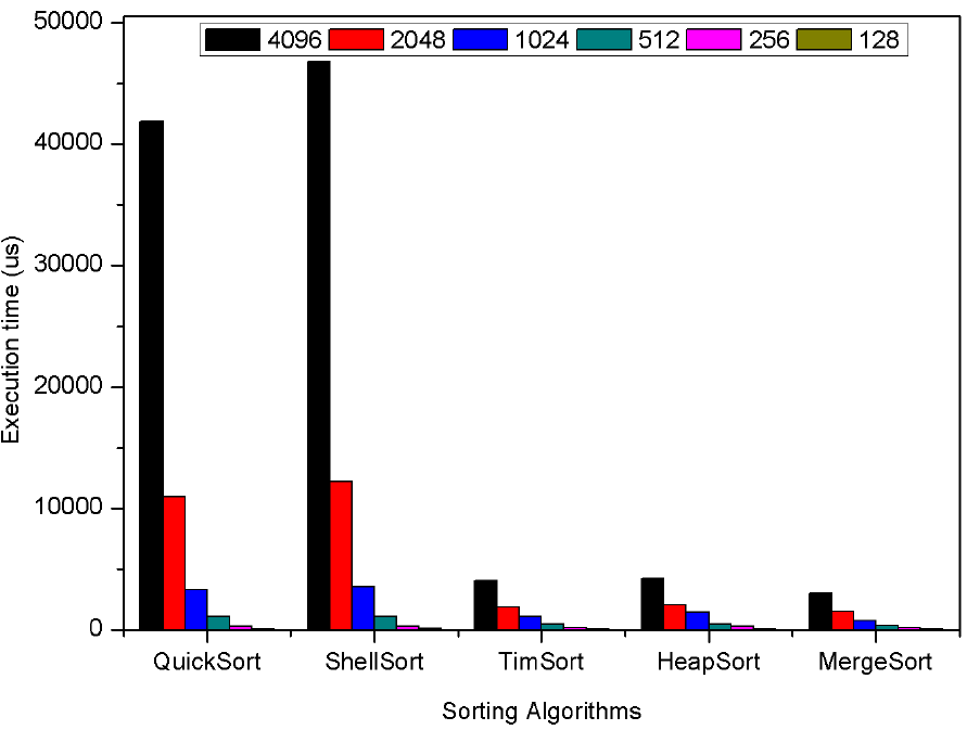
Fig. 12 Execution time of the HeapSort, QuickSort, MergeSort, ShellSort et TimSort algorithms on a processor
Second, we compared the performance of the sorting algorithms in terms of standard deviation as shown in table 4, which illustrates the standard deviation for each algorithm. Finally, we calculated the different resource utilization for the sorting algorithms (Table 5) and we noted that BubbleSort, InsertionSort and SelectionSort consume less of a resource. In contrast, ShellSort is the best algorithm in terms of resource utilization (Slice, LUT, FF and BRAM) (Figure 14, 15) because BubbleSort, InsertionSort and SelectionSort have an important complexity. From the results, it is concluded that MergeSort is the best algorithm.
Table 4 Standard deviation of different algorithms
| BubbleSort | InsertionSort | HeapSort | MergeSort | QuickSort | SelectionSort | ShellSort | TimSort | |
|---|---|---|---|---|---|---|---|---|
| 8 | 2753 | 2173 | 3636 | 3198 | 2989 | 2486 | 2770 | 2911 |
| 16 | 4786 | 3654 | 4524 | 4102 | 4413 | 3941 | 4410 | 3660 |
| 32 | 7310 | 5671 | 6075 | 6713 | 6301 | 9772 | 6123 | 6400 |
| 64 | 112167 | 9209 | 23719 | 9919 | 58629 | 9895 | 69133 | 10317 |
| 128 | 36686 | 10277 | 13835 | 7573 | 13875 | 42599 | 104016 | 10721 |
| 256 | 182061 | 302001 | 557507 | 19687 | 431402 | 83059 | 74621 | 75778 |
| 512 | 844048 | 757201 | 168523 | 116047 | 757716 | 284322 | 389055 | 782516 |
| 1024 | 2519380 | 676104 | 1239939 | 409297 | 437650 | 1854144 | 1362460 | 1164588 |
| 2048 | 4825091 | 1993282 | 210328 | 85225 | 2207375 | 2400166 | 585655 | 243134 |
| 4096 | 9895405 | 3179333 | 756228 | 159427 | 3462193 | 6339409 | 1431203 | 539362 |
Table 5 Utilization resources of the sorting algorithms
| Slices | LUT | FF | BRAM | |
|---|---|---|---|---|
| BubbleSort | 57 | 173 | 159 | 2 |
| InsertionSort | 55 | 183 | 132 | 2 |
| SelectionSort | 95 | 306 | 238 | 2 |
| ShellSort | 107 | 321 | 257 | 2 |
| QuickSort | 188 | 546 | 512 | 6 |
| HeapSort | 211 | 569 | 576 | 2 |
| MergeSort | 278 | 706 | 797 | 6 |
| TimSort | 998 | 3054 | 2364 | 69 |


After that, we used HLS directives in order to improve the performance of the different algorithms. We calculated the execution time for each optimized Hardware implementation of sorting algorithms. We compared those algorithms using different sizes of the array (8-4096) and several permutations (47 permutations) and vectors (47 vectors) which are generated using a generator of permutations proposed by Lehmer encoded in 32 and 64 bits to analyze the performance of each algorithm. Hence, we talk about multicriteria sorting for use in real-time decision support systems.
We calculated the execution time of the sorting algorithms for different sizes of arrays ranging from 8 to 4096 elements. The permutations are generated using the Lehmer code and encoded in 4 or 8 bytes. Table 6 and table 7 report the minimum, average and maximum execution time for each algorithm in 4 bytes and 8 bytes respectively. Figure 16 shows the execution time of the sorting algorithms for the average cases using elements encoded in 4 bytes. When N is smaller than 64, we display a zoom from the part framed red. Hence, SelectionSort is 1.01x-1.23x faster than the other sorting algorithms if N ≤ 64.
Table 6 Execution time of the sorting algorithms encoded in 4bytes of us
| BubbleSort (US) | InsertionSort (US) | SelectionSort (US) | ShellSort (US) | QuickSort (US) | HeapSort (US) | MergeSort (US) | TimSort (US) | |||||||||||||||||
|---|---|---|---|---|---|---|---|---|---|---|---|---|---|---|---|---|---|---|---|---|---|---|---|---|
| Min | Avg | Max | Min | Avg | Max | Min | Avg | Max | Min | Avg | Max | Min | Avg | Max | Min | Avg | Max | Min | Avg | Max | Min | Avg | Max | |
| 8 | 11.244 | 17.302 | 23.181 | 11.036 | 17.106 | 22.98 | 10.78 | 16.84 | 22.29 | 11.816 | 17.88 | 23.768 | 12.55 | 18.68 | 24.6 | 11.903 | 17.99 | 23.8 | 12.84 | 18.93 | 24.847 | 12.12 | 18.12 | 24 |
| 16 | 15.934 | 22.009 | 27.897 | 14.11 | 20.206 | 26.102 | 13.914 | 20 | 25.88 | 16.1 | 22.25 | 28.1 | 17.16 | 23.22 | 29.11 | 15.77 | 21.85 | 27.73 | 17.52 | 23.6 | 29.5 | 16 | 22.07 | 27.95 |
| 32 | 32.317 | 38.763 | 44.647 | 24.02 | 30.15 | 36.03 | 23.85 | 29.9 | 35.25 | 27.12 | 33.25 | 39.14 | 28.3 | 34.3 | 40.2 | 24.97 | 31.1 | 37.02 | 28.36 | 34.48 | 40.36 | 27.51 | 31.18 | 37 |
| 64 | 97.11275 | 103.255 | 109.136 | 59.44 | 65.56 | 77.185 | 59.13 | 65.25 | 71.13 | 54.12 | 60.24 | 66.12 | 59.6 | 62.8 | 68.6 | 46.66 | 52.78 | 58.66 | 52.33 | 58.465 | 64.34 | 44.8 | 50.89 | 56.7 |
| 128 | 348.937 | 358.255 | 360.94 | 190.94 | 196.96 | 202.84 | 191 | 197.2 | 203 | 120.2 | 126.3 | 132.1 | 131.7 | 137.9 | 143.7 | 96.535 | 102.665 | 108.54 | 105.71 | 111.88 | 117.76 | 88.39 | 94.5 | 100.3 |
| 256 | 1344.71 | 1350.84 | 1356.72 | 708.1 | 714.21 | 720.039 | 701 | 707.2 | 713 | 281.8 | 293.55 | 293.8 | 342.7 | 351.2 | 357.07 | 222.47 | 228.57 | 234.45 | 223.1 | 231.3 | 237.25 | 182.9 | 189 | 197.9 |
| 512 | 5304.07 | 5310.11 | 5315.92 | 2711.18 | 2717.29 | 2723.17 | 2698.4 | 2711.4 | 2717.1 | 662.16 | 668.2 | 674.1 | 984.1 | 1001.3 | 1007 | 459.92 | 466.05 | 471.93 | 476.4 | 782.5 | 788.4 | 387 | 393.17 | 399 |
| 1024 | 21095.1 | 21101.2 | 21107.01 | 10629.9 | 10635.7 | 10645.4 | 10649 | 10655 | 10661.1 | 1607.6 | 1625.1 | 1803 | 2881 | 3121 | 3127 | 1001.8 | 1015.5 | 1024.6 | 1025.4 | 1031.5 | 1037.4 | 826.75 | 832.85 | 837.2 |
| 2048 | 32767 | 83852.9 | 84177.8 | 31733.1 | 42209.7 | 42215.5 | 32767 | 42288 | 42294 | 4021.6 | 4027.67 | 4033.48 | 4232 | 10660 | 10665 | 2221.04 | 2227.1 | 2233 | 2182.1 | 2211.5 | 2217.3 | 1763.4 | 1769.5 | 1775 |
| 4096 | 32767 | 333077 | 336274.5 | 31744.8 | 168307 | 168313 | 32767 | 168531 | 168536 | 9750.4 | 9756.4 | 9762 | 20630 | 101507 | 101512 | 4810.5 | 4848.5 | 4854.2 | 4728.9 | 4734.9 | 4740.7 | 3750.1 | 3756 | 3761.9 |
Table 7 Execution time of the sorting algorithms encoded in 8bytes of us
| BubbleSort (US) | InsertionSort (US) | SelectionSort (US) | ShellSort (US) | QuickSort (US) | HeapSort (US) | MergeSort (US) | TimSort (US) | |||||||||||||||||
|---|---|---|---|---|---|---|---|---|---|---|---|---|---|---|---|---|---|---|---|---|---|---|---|---|
| Min | Avg | Max | Min | Avg | Max | Min | Avg | Max | Min | Avg | Max | Min | Avg | Max | Min | Avg | Max | Min | Avg | Max | Min | Avg | Max | |
| 8 | 11.312 | 17.447 | 23.385 | 11.042 | 17.15 | 22.95 | 10.94 | 17.01 | 22.88 | 11.92 | 18 | 23.87 | 12.56 | 18.67 | 24.57 | 11.87 | 17.96 | 23.85 | 12.79 | 18.89 | 24.78 | 12.12 | 18.13 | 24.01 |
| 16 | 16.32 | 22.419 | 28.341 | 14.38 | 20.48 | 26.37 | 14.36 | 20.5 | 26.48 | 16.2 | 22.5 | 28.5 | 17.4 | 23.5 | 29.38 | 16.048 | 22.16 | 28.08 | 17.91 | 24.02 | 29.91 | 16.38 | 22.43 | 28.29 |
| 32 | 33.433 | 39.53 | 45.416 | 24.73 | 30.82 | 36.69 | 24.55 | 30.31 | 36.5 | 27.8 | 33.9 | 39.78 | 28.9 | 34.9 | 40.8 | 25.673 | 31.76 | 37.636 | 28.95 | 35.05 | 40.9 | 25.74 | 31.8 | 40.86 |
| 64 | 98.482 | 104.75 | 110.45 | 60.79 | 66.89 | 72.03 | 60.5 | 66.61 | 72.48 | 55.49 | 61.57 | 67.47 | 58 | 64.14 | 70.02 | 48.05 | 54.15 | 60.027 | 53.75 | 59.86 | 65.74 | 46.18 | 52.28 | 58.14 |
| 128 | 353.24 | 359.35 | 365.236 | 193.64 | 199.75 | 205.63 | 193.8 | 199.9 | 205.8 | 123 | 129.1 | 135 | 134.6 | 140.6 | 146.5 | 99.36 | 105.47 | 111.35 | 108.4 | 114.5 | 120 | 91.22 | 97.3 | 103.21 |
| 256 | 1350.31 | 1356.42 | 1362.3 | 710.56 | 717.07 | 802.5 | 704.7 | 718.2 | 724.1 | 292.9 | 299 | 304.9 | 345.5 | 351.7 | 357.5 | 222.47 | 228.57 | 234.45 | 228.1 | 234.45 | 240.12 | 188.5 | 194.5 | 200.4 |
| 512 | 5315.43 | 5321.45 | 5327.25 | 2722.62 | 2728.8 | 2716.5 | 2722.5 | 2728.6 | 2735.6 | 670.4 | 676.6 | 682.5 | 482.5 | 489 | 494.8 | 471.27 | 477.38 | 484.32 | 484.7 | 490.8 | 496.7 | 398.3 | 404.5 | 410.3 |
| 1024 | 20926.15 | 21243.01 | 21140.12 | 10652.9 | 10656.11 | 10664.8 | 10672 | 10678.2 | 10684 | 1642.5 | 1648.7 | 1654.6 | 2893 | 3132.8 | 3138.7 | 1035.47 | 1041.58 | 1047.7 | 1048.1 | 1054.2 | 1060.1 | 849.6 | 855.7 | 861.8 |
| 2048 | 32767 | 84217.69 | 84223.49 | 31734.6 | 41802.5 | 42264.7 | 32767 | 41525.3 | 46392 | 4067 | 4073 | 4078.8 | 4254.9 | 10682 | 10688 | 2244.7 | 2272.5 | 2278.43 | 2250.9 | 2257 | 2262.9 | 1809 | 1815 | 1821 |
| 4096 | 32767 | 336356 | 336361.8 | 30728 | 168554 | 168578 | 32767 | 168618 | 168624 | 9814 | 9820.5 | 9826.3 | 67153 | 38599 | 38684 | 4930 | 4936.1 | 4941.95 | 4812.4 | 4819.5 | 4825.3 | 3837 | 3843.9 | 3849.7 |

Otherwise, Figure 17 shows the execution time of the sorting algorithms when N > 64. We note that BubbleSort, InsertionSort, SelectionSort and QuickSort have a high execution time. Thereafter, we compared only the other four algorithms to choose the best algorithm in terms of execution and standard deviation. In addition, we calculated the standard deviation for the different sorting algorithms when N ≤ 64. Tables 8 and 9 show that the standard deviation is almost the same. Since we rejected the BubbleSort, InsertionSort, SelectionSort and QuickSort algorithms if N > 64, we compared the standard deviation and execution time between HeapSort, MergeSort, ShellSort and TimSort. Consequently, TimSort has the best standard deviation with N ≤ 64 and N > 64 as shown in table 9 and Fig 18.

Table 8 Standard deviation for sorting algorithms (N ≤ 64)
| BubbleSort | InsertionSort | SelectionSort | QuickSort | HeapSort | MergeSort | ShellSort | TimSort | |
|---|---|---|---|---|---|---|---|---|
| 8 | 3.47244 | 3.474 | 3.485 | 3.504 | 3.486 | 3.491 | 3.4752 | 3.471 |
| 16 | 3.4789 | 3.481 | 3.507 | 3.4849 | 3.4777 | 3.483 | 3.4742 | 3.4712 |
| 32 | 3.474 | 3.474 | 3.476 | 3.4757 | 3.475 | 3.4749 | 3.4763 | 3.4731 |
| 64 | 3.475 | 3.4743 | 3.4762 | 3.4739 | 3.474 | 3.475 | 3.4747 | 3.4724 |
Table 9 Standard deviation for sorting algorithms with N > 64
| HeapSort | MergeSort | ShellSort | TimSort | HeapSort | MergeSort | ShellSort | TimSort | |
|---|---|---|---|---|---|---|---|---|
| 128 | 3.475 | 3.4752 | 3.4745 | 3.4736 | 3.486 | 3.491 | 3.4752 | 3.471 |
| 256 | 3.474 | 3.4737 | 3.4758 | 3.4731 | 3.4777 | 3.483 | 3.4742 | 3.4712 |
| 512 | 3.6695 | 3.707 | 3.472 | 3.4714 | 3.475 | 3.4749 | 3.4763 | 3.4731 |
| 1024 | 4.082 | 3.479 | 3.56 | 3.4714 | 3.474 | 3.475 | 3.4747 | 3.4724 |

Figure 18 shows the execution time of Timsort, MergeSort, HeapSort and ShellSort algorithms for the average case. For example, when N=4096, the execution time was 3756us, 4734.9us, 4848.5us and 9756.4us for Timsort, MergeSort, HeapSort and ShellSort respectively. For a large number of elements, we concluded that TimSort was 1.12x-1.21x faster than MergeSort, 1.03x-1.22x faster than HeapSort and 1.15x-1.61x faster than ShellSort running on FPGA (Figure 21). Table 7 presents the execution time for each algorithm using several elements encoded in 8 bytes. The obtained results show almost the same results obtained when using elements encoded in 4 bytes. From table 6 and 7, it is observed that the results obtained for TimSort in table 6 and 7 have a smaller execution time in each case. Thus, the performance of the sorting algorithms depends on the permutation or vectors.
Moreover, we notice that the computational execution time of 6 and 7 in hardware implementation is reduced compared that in processor Intel (Table 3) when the same frequency is used. For example, when N=2048, the hardware implementation was 1815 us (50 MHz) and the software implementation was 61,926 us (2260 MHz) for Timsort. We study two cases where the frequency is 2260Mhz the execution time is 61.926 us. In contrast, if the frequency decreases to 50MHz then the execution time increases and for this reason, we notice that the time on FPGA is very faster if the frequency is 50MHz.
From Software and Hardware implementation, we concluded that BubbleSort, InsertionSort and SelectionSort have an important execution time for a large number of elements. In addition, we concluded that MergeSort is the best algorithm in software execution and TimSort in the FPGA when N > 64; otherwise, we note that InsertionSort much faster than the other algorithms running on the processor and faster than SelectionSort running in the hardware platform. Table 10 shows the different resources utilization for BubbleSort, InsertionSort, SelectionSort, HeapSort, Merge-Sort, ShellSort and TimSort. We can see that Tim sort consumes more resources than the other algorithms. TimSort consumed 44% more for Slice LUT in hardware implementation and around 9 % for Slice Register. We concluded that when we increase the performance of the algorithm in terms of execution time, then we increase the amount of available the number of available resource utilization on the FPGA.
Table 10 Utilization of resources of the sorting algorithms
| BubbleSort | InsertionSort | SelectionSort | ShellSort | QuickSort | HeapSort | MergeSort | TimSort | |||||||||||||||||
|---|---|---|---|---|---|---|---|---|---|---|---|---|---|---|---|---|---|---|---|---|---|---|---|---|
| LUT | FF | BRAM | LUT | FF | BRAM | LUT | FF | BRAM | LUT | FF | BRAM | LUT | FF | BRAM | LUT | FF | BRAM | LUT | FF | BRAM | LUT | FF | BRAM | |
| 8 | 242 | 121 | 1 | 219 | 131 | 0 | 336 | 203 | 1 | 356 | 224 | 0 | 733 | 541 | 2 | 524 | 444 | 0 | 955 | 877 | 0 | 5299 | 2480 | 35 |
| 16 | 176 | 136 | 1 | 226 | 139 | 0 | 333 | 214 | 1 | 355 | 232 | 0 | 750 | 552 | 2 | 526 | 459 | 1 | 985 | 883 | 0 | 5326 | 2498 | 35 |
| 32 | 189 | 136 | 1 | 187 | 115 | 0.5 | 351 | 225 | 1 | 314 | 208 | 0.5 | 776 | 564 | 2 | 541 | 474 | 1 | 856 | 809 | 1.5 | 5293 | 2482 | 35 |
| 64 | 199 | 149 | 1 | 201 | 123 | 0.5 | 363 | 236 | 1 | 319 | 216 | 0.5 | 814 | 608 | 2 | 556 | 489 | 1 | 871 | 815 | 1.5 | 5320 | 2499 | 35.5 |
| 128 | 215 | 162 | 1 | 212 | 131 | 0.5 | 373 | 247 | 1 | 337 | 224 | 0.5 | 820 | 588 | 2 | 583 | 504 | 1 | 885 | 821 | 1.5 | 5487 | 2516 | 35.5 |
| 256 | 228 | 175 | 1 | 221 | 139 | 0.5 | 365 | 258 | 1 | 345 | 232 | 0.5 | 835 | 600 | 2 | 606 | 519 | 1 | 893 | 827 | 1.5 | 5468 | 2535 | 35 |
| 512 | 238 | 188 | 1 | 239 | 147 | 0.5 | 394 | 269 | 1 | 359 | 240 | 0.5 | 841 | 612 | 2 | 611 | 534 | 1 | 925 | 849 | 1.5 | 5494 | 2552 | 35.5 |
| 1024 | 245 | 201 | 1 | 248 | 155 | 1 | 407 | 280 | 1 | 365 | 248 | 1 | 860 | 624 | 3 | 651 | 551 | 1 | 936 | 855 | 3 | 5545 | 2569 | 36 |
| 2048 | 259 | 216 | 2 | 265 | 163 | 2 | 418 | 293 | 2 | 367 | 258 | 2 | 909 | 638 | 6 | 669 | 566 | 2 | 942 | 861 | 6 | 5668 | 2586 | 38 |
| 4096 | 291 | 229 | 4 | 274 | 171 | 4 | 434 | 304 | 4 | 384 | 266 | 4 | 976 | 682 | 15.5 | 689 | 581 | 4 | 954 | 867 | 12 | 5841 | 2602 | 44 |
7 Conclusion
In this paper, we presented the optimized hardware implementation of sorting algorithms to improve the performance in terms of execution time using a different number of elements (8-4096) encoded in 4 and 8 bytes. We used a High-Level Synthesis tool to generate the RTL design from behavioral description. However, we used a muli-criteria sorting algorithms which contain several actions in line and different criteria in columns.
A Comparative analysis of the various results obtained by these sorting algorithms was done based on two different cases (software and optimized hardware) and two parameters (Execution time and resource utilization) on a Zynq-7000 platform. From the results, it is concluded that BubbleSort, InsertionSort and QuickSort have a high execution time. In addition, TimSort ranges from 1.12x-1.21x faster than MergeSort, 1.03x-1.22x faster than HeapSort and 1.15x-1.61x faster than ShellSort when N ≥ 64 and using optimized hardware with many permutations/vectors. In contrast, when N < 64, Selection sort is 1.01x-1.23x faster than the other sorting algorithms.
As future work, we plan to use the hardware TimSort algorithm in the avionics field and in the hardware implementation of a decisional system. The next step is to include the best solution in hardware path planning algorithms.

