1 Introduction
For building a depth map with a monocular camera its location for a set of frames must be known, photo-consistency must be satisfied and the images must have texture. However, real environments present changes in light conditions and low-texture, very reflective or translucent objects. These facts break the Lambertian condition (photo-consistency) and affects the photometric error estimation reducing the accuracy of the estimated depth maps. The regularizer term in a variational framework tackles this problem to some extent, but under difficult conditions, the estimations still have low accuracy.
One alternative is to include information of a known object in the scene (shape prior). In this sense, we propose to optimize a model w.r.t. shape, pose and scale and then include depth data of the shape prior seen from the estimated camera pose. This data integration is done using also variational methods and the primal dual algorithm, achieving a denoised and enhanced depth map, especially in the region of the selected object.
The main contributions of this work are as follows. (1) The coupling of four modules: a module for tracking the camera based on keyframes, bundle adjustment and ORB features called ORB-SLAM2; a module for dense mapping based on a photometric error, a regularizer and a decoupling term; a module for estimating the optimal 3D model that best fits to observed data based on Gaussian Process Latent Variable Models GPLVM ; a module for denoising, inpainting and depth merging based on variational methods. (2) A novel variational formulation that integrates in one algorithm both the module for dense mapping with monocular camera and the module for depth merging using a shape prior. (3) The experiments carried out in order to quantify the improvements in depth accuracy.
This paper is structured as follows. In section II we describe related work. In section III we present the proposed methodology: initial depth map estimation, depth refinement using variational methods, shape prior estimation, integration of depth data of the optimal model (shape prior) for enhancing the estimated depth map in sequential (depth map building followed by shape prior integration) and simultaneous way (depth map building and shape prior integration at the same time). Finally, we present the results and conclusions in section IV and V, respectively.
2 Related Work
Two techniques for minimizing the energy functional in the process of building a depth map with a monocular camera stand out. The technique of sequential convex optimization linearises the photometric error, as is explained in [20], so the camera motion must be small.
A coarse-to-fine scheme with a pyramid of several levels is built to copy with fast camera motion. This technique was successfully implemented in the work of dense mapping of [18]. The other technique, the non-convex variational one, based on optical flow for long displacements [17], uses an auxiliary variable that decouples the cost function into two terms. The regularizer term is solved with the primal-dual algorithm [1], [21], and the photometric term is solved by exhaustive search over a finite range of discrete values of the inverse depth. This technique was implemented in the work of dense localization and dense mapping of [12].
In order to improve the accuracy of depth maps created with a monocular camera, a shape prior that considers the scene with box-like structures, with extensive low-texture surfaces like walls, ceilings and floors, can be used. This scene shape prior allows to improve the whole scene. For example, the system [13] estimates depth maps using a monocular camera in workspaces with large plain structures like floors, walls or ceilings. The curvature of a second order approximation of the data term at the minimum cost defines the reliability of the initial depth, getting good depth estimates at the borders of bland objects (high curvature). Good depth data is propagated to an interior pixel (inpainting) from the closest valid pixels along the main 8 star directions by using a non-local high-order regularization term, in a variational approach, that favours solutions with affine surfaces (prior). The energy is minimized in straight way with the primal-dual algorithm.
The system [3] shows outstanding performance in low-textured image regions and for low-parallax camera motion. It includes a term, besides the data term and regularization term, that depends on three scene priors: planarity of homogeneous color regions (using superpixels), the repeating geometry primitives of the scene (data-driven 3D primitives learned from RGBD data), and the Manhattan structure of indoor rooms (layout estimation and classification of box-like structures). The scene prior terms model the distance from every point to its estimated planar prior. The energy is minimized using a variational approach with a coupling term, the primal-dual algorithm and exhaustive search. In contrast to [13], it requires a preprocessing step.
Other kind of shape prior, the object-based one, is also used for 2D segmentation, 3D reconstruction and point cloud refinement. The monocular system [14] uses DCT for compressing the 3D level-set embedding functions and GPLVM for nonlinear dimensionality reduction to capture shape variance.
The energy function measures the discrepancy between the projected 3D model into the image plane and the probabilistic 2D occupancy map that defines the foreground of the observed object in the image (image-based energy). The minimization is done w.r.t. pose and shape of the 3D model. A 2D segmentation results automatically after convergence. The system [4] also uses DCT, GPLVM, and a monocular camera but unlike [14] it builds depth maps minimizing the photo-consistency error with variational methods and PTAM [7] for camera tracking and fuses them into a volumetric grid through time.
The main goal is to improve the dense reconstruction by replacing the TSDF values of the optimal model in the volumetric grid in a straight way. Moreover, the energy function combines image and depth data for pose, shape and scale optimization (image and depth-based energy). The system [9] removes point cloud artifacts like noisy points, missing data and outliers using a learned shape prior. Besides using DCT and GPLVM as [4, 14], it uses part-based object detector [5] for detecting the object in the scene, VisualSFM [19] for performing structure from motion and getting a point cloud that represents the scene, SAC-segementation for segmenting the point cloud into the region of the object, and iterative optimization of an energy function that depends on the evaluation the point cloud into the embedding function (depth-based energy). The shape prior is finally used for enhancing the accuracy and the completeness of the estimated 3D representation.
Our system uses, like in [12], an auxiliary variable that decouples the data term and the regularization term. The solution is found with the primal-dual algorithm and exhaustive search. We employ object shape priors like [4, 9], but instead of modifying a point cloud like [9] or a volumetric structure directly like [4], we enhance the built depth maps by merging a synthetic depth map coming from the shape prior using a novel variational formulation that considers an additional term for the shape prior data, like is done in [3, 13], and exploiting the ideas of [8] where color aerial images are fused considering the redundant information of the scene.
Finally, we propose to couple both modules (depth map creation and shape prior integration) in just one module, considering a known shape prior previous to build the depth map.
3 Methodology
The main pipeline of the system is shown in fig. 1. An initial depth map is estimated by minimizing the photometric error gathered from a set of images with the camera pose estimated with ORB-SLAM2. This coarse depth map is refined using a variational framework with an energy functional made up of a data term, a regularizer term and an additional decoupling term. The primal-dual algorithm and exhaustive search are employed in an alternating fashion for solving this problem.

Fig. 1 Main pipeline of the proposed system. The resulting depth map integrates depth data from the optimal model (shape prior)
We use DCT for compressing the 3D models of the object of interest represented as 3D level sets embedding functions, GPLVM for dimensionality reduction and Levenberg-Marquart for minimizing the discrepancy between a model hypothesis and depth data of the segmented region of the object, having as argument its shape, pose and scale.
The optimal model is used for creating a synthetic depth map by reading the depth buffer of its explicit representation in OpenGL, seen from the estimated camera pose. The synthetic depth map is merged with the built depth map using a novel variational formulation. Finally, a variant in this formulation is presented for making simultaneously depth map building and shape prior integration.
3.1 Building an Initial Depth Map
A 3D point in the reference frame
where
This 3D point is projected into the image plane
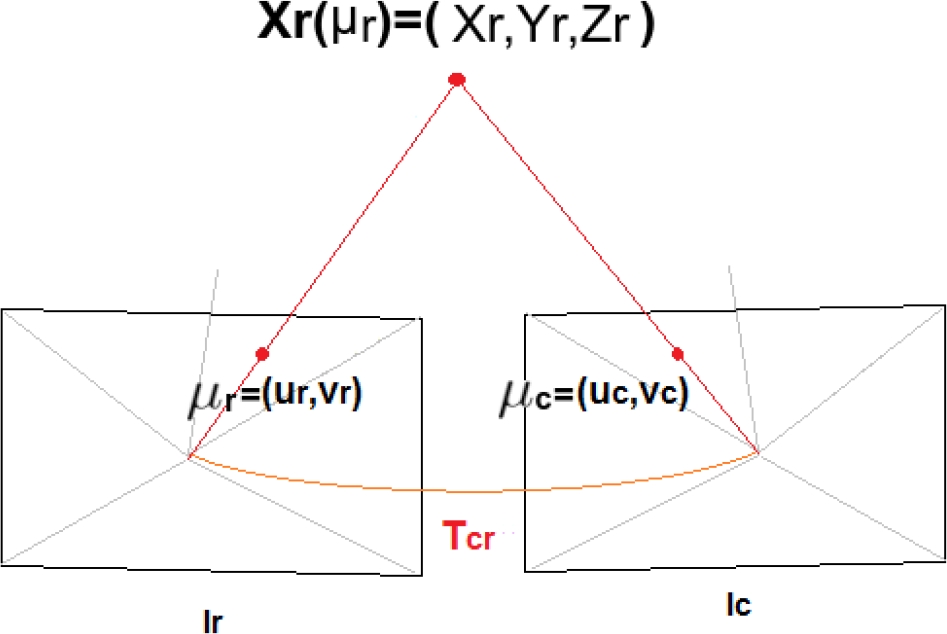
Fig. 2 Projection of a 3D point referenced to the coordinate system
If the same process is carried out for all the pixels of the reference image, a
synthetic image that represents the scene observed from the pose defined by the
transformation matrix
However, the inverse depth of the pixel
where the projected image
as
where
In real environments, there are changes in light conditions, which break the assumption of photo-consistency and the estimations are affected drastically. Besides, images of real scenes present regions with low texture that generate depth estimations in the most dominated by noise [2]. All these problems are reduced to some extent when using a regularizer in a variational framework.
3.2 Refining the Initial Depth Map with Variational Methods
A variational approach [16] is
adopted for smoothing the depth map, preserving discontinuities and increasing
the robustness of the algorithm against illumination changes, occlusions and
noise. It was proposed first by Ruding, Osher and Fatemi ROF to consider the
“Total Variation” as a regularizer
where
where
The
reducing the regularity strength where the edge magnitude is high, therefore decreasing the smoothing effect in boundaries. The problem of computing the inverse depth map becomes:
where
3.2.1 The Decoupling Approach
In order to solve (12), we use
the iterative primal-dual algorithm described in [12] for depth map building. This algorithm requires
both the regularizer and the data term to be convex. However the last term
is not a convex function. One solution to this problem is to decouple both
terms and solve the decoupled version instead of the original one. The
advantage of the decoupling approach is that it allows us to independently
solve for the regularizer term using convex optimization methods and for the
data term using a simple exhaustive search. The decoupling approach is based
on eliminating the constraint
where
enforcing
correspond to the TV-ROF denoising problem, defined in eq. (8). It is convex in
where
In our case, the convex functions are
where
Replacing
We do a step of projected gradient ascent (maximization problem) for the dual
variable
where
The primal-dual algorithm and the exhaustive search are alternated and
3.3 Tracking the Monocular Camera
For tracking the camera we use ORB-SLAM2 [11] with RGB-D inputs. It builds globally consistent sparse reconstructions for long-term trajectories with either monocular, stereo or RGB-D inputs, performing in real time on standard CPUs and including loop closure, map reuse and relocalization. This system has three main parallel threads: the tracking with motion only bundle adjustment (BA), the local mapping with local BA, and the loop closing with pose graph optimization and full BA. It does not fuse depth maps but uses ORB features for tracking, mapping and place recognition tasks. With BA and keyframes, it achieves more accuracy in localization than state-of-the-art methods based on ICP or photometric and depth error minimization. Place recognition, based on bag of words, is used for relocalization in case of tracking failure.
3.4 Shape Prior Estimation
In order to estimate the 3D model (shape prior) that best fits to depth data associated to an object of interest in the scene, we minimize the discrepancy between a model hypothesis and observed depth data back projected from the segmented region of the object. We evaluate the resulting point cloud in a 3D level-set embedding function that encodes the object model implicitly. This alignment consist in reducing the distance of the points to the zero-level of the embedding function having as arguments the pose, scale and shape (latent variable), using Levenberg-Marquardt.
Initially, the
The Latent variable Model LVM is used for dimensionality reduction, to capture
the shape variance as low dimensional latent shape spaces. The dimensionality
reduction is applied to DCT coefficients such that the resulting latent
variables have 2 dimensions instead of
The mapping is modeled using a Gaussian process that defines areas where there are high certainty of getting a valid shape. Next, the latent variable that best fits to depth data is searched over a continuous space (no just the ones used for learning) and the coefficients associated to it are estimated.
The 3D level-set embedding function encoded in the coefficients is computed with the inverse discrete cosine transform IDCT. Besides shape optimization, the pose and scale of the 3D model are optimized in alternating way, using initially a coarse estimation of pose and scale, computed with depth data of the object and assuming that the car is over a flat surface. For model pose we use Lie algebra instead of Rodrigues notation for rotations.
3.5 Shape Prior Integration
Following a similar process for solving the minimization problem of the regularizer term and decoupling term of eq. (16), we minimize the energy:
where
where
where
We propose to use the scheme of [8]
(where color images for aerial applications are merged, denoised and inpainted)
for merging depth data of two sources, getting an enhanced depth map. The
iterative optimization corresponds to perform in alternating way gradient ascent
over the dual variables and gradient descent over the primal variable
where
Following the algorithm 1 of [1]
and the parameter setting of [8]
we set the primal and dual time steps with
3.6 Putting together Depth Map Estimation and Shape Prior Integration
The algorithms previously described for building a depth map with a monocular camera and for integrating the shape prior are based on variational techniques that are solved with the primal-dual algorithm so they share common modules. Moreover, the object of interest is static and rigid so its pose, scale and shape do not change with time. We exploit these facts for implementing one algorithm that takes a shape prior estimated previously (for example in a previous keyframe) and makes simultaneously depth map building and shape prior integration. Now, we integrate shape prior data into the energy functional (9) with an additional term, the shape prior term:
where
where
where
where
4 Results
We carry out three experiments: one with synthetic data for computing the accuracy of
the estimated depht map and the other ones with real data for enhancing the created
depth map with shape priors and variational methods. For the first experiment we use
40 images
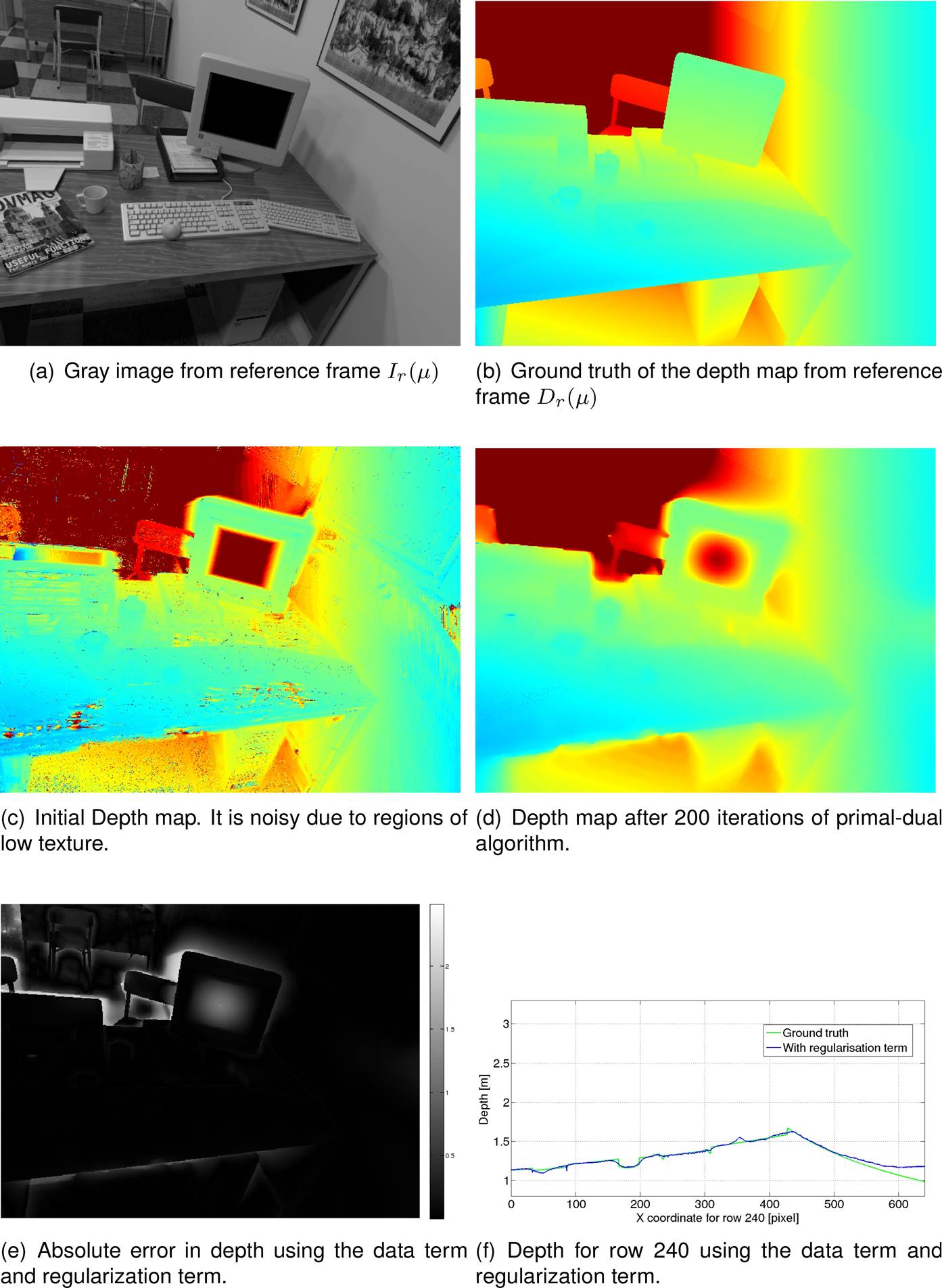
Fig. 3 (a) Gray image from reference frame, (b) ground truth of the depth map from reference frame, (c) initial depth map built using the photometric error, (d) refined depth map after 200 iterations of primal-dual algorithm, (e) absolute error of the solution and (f) depth for row 240 compared to ground truth
For the second and third experiments the kinect 1.0 is employed: the RGB images for
building a depth map and the depth map coming from the sensor as reference for
estimating the accuracy of the solution. We use 40 images
Figures 4(a) and 4(b) show the image of reference in gray and the depth coming from the
sensor. Figures 4(c) and 4(d) show the initial depth map obtained by minimizing eq. (7) and the refined depth map after
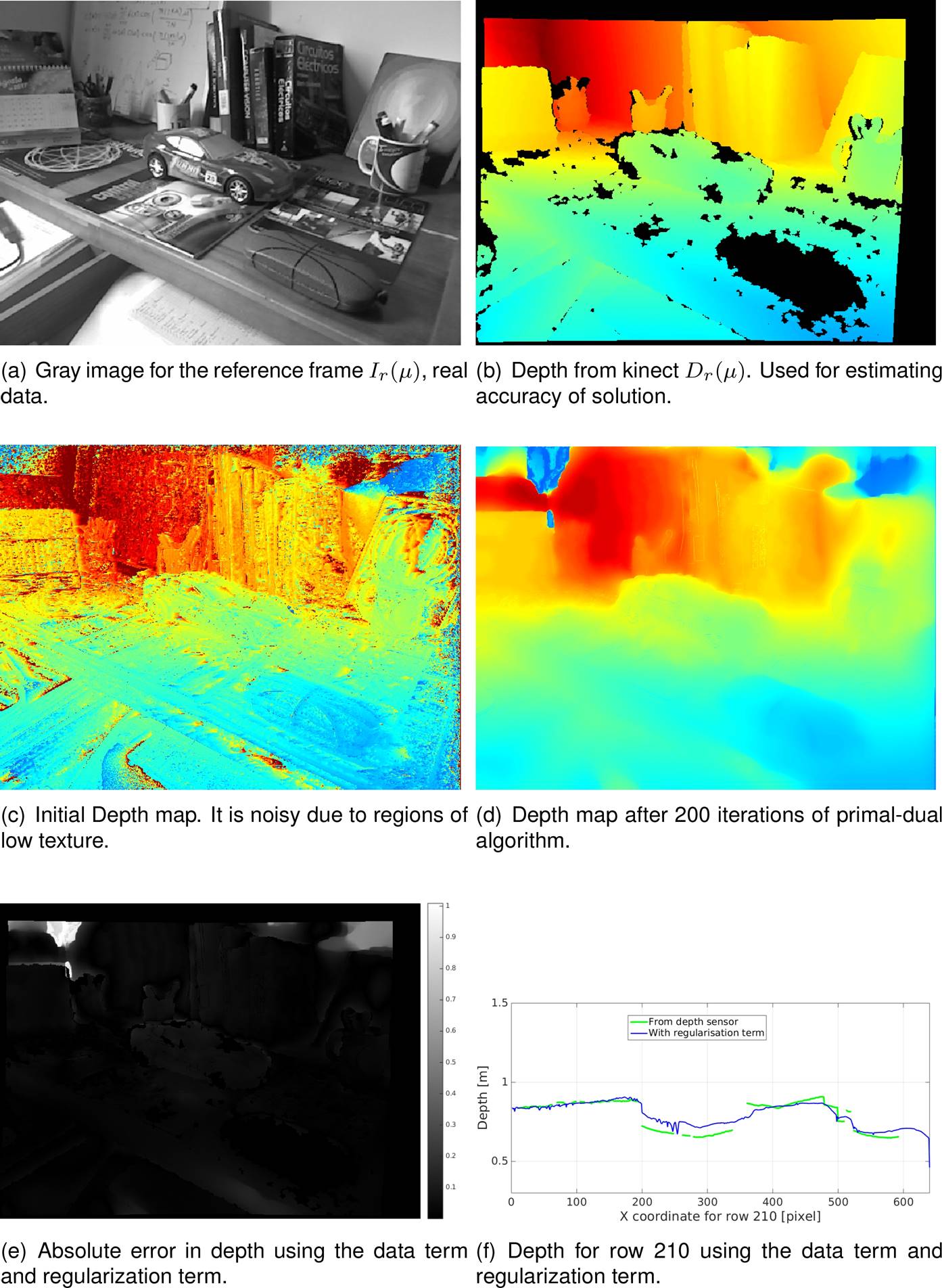
Fig. 4 (a) Gray image from reference frame (real data), (b) depth got with kinect sensor for reference frame (used for estimating depth accuracy of solution), (c) initial depth map built using the photometric error, (d) refined depth map after 200 iterations of primal-dual algorithm, (e) absolute error of the solution and (f) depth for row 210 compared to ground truth
Next, we manually segment the car (see fig 5(a))
and compute a point cloud (red points in fig.
5(b)) with the depth data of the built depth map in the segmented area.
This point cloud is aligned with a 3D model by minimizing an energy function w.r.t.
pose, scale and shape. For an initial estimation of position we use the centroid of
the point cloud, adding
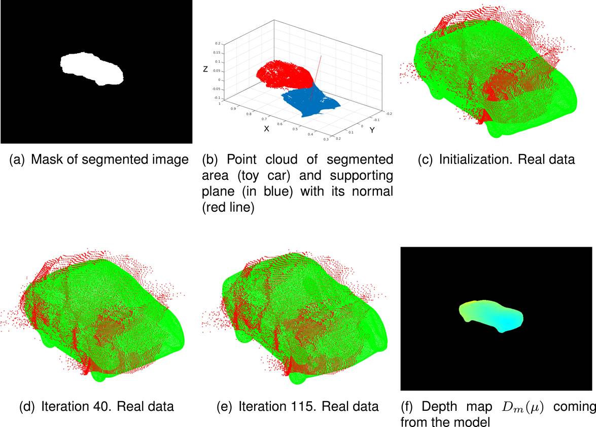
Fig. 5 Steps in the process for estimating the optimal 3D model and a synthetic depth map from the current camera pose. (a) Mask of the segmented car, (b) Point cloud of the segmented car and supporting plane, (c) Initial state of the 3D model, (d) 3D model for iteration 40, (e) 3D model for iteration 115 and (f) depth map from the model
For the scale we consider the average distance of each point to the centroid. We
suppose a supporting plane (blue points in fig.
5(b)) in order to estimate two of the three angles that define the
initial orientation of the car. The third angle is found with exhaustive search.
Summarizing, the initial position is
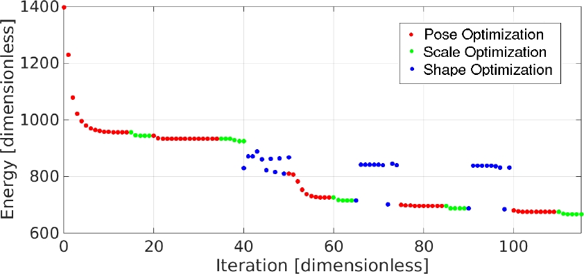
For refining the initial estimation we carry out two cycles with the sequence: 15
iterations for pose and 5 iterations for scale. At the end of this sequence, 40
iterations have been done and very close pose and scale estimations are obtained
(see fig. 5(d)). With these estimations we can
perform exhaustive search over the
The final position is
Once we have two depth maps: one from the optimal 3D model and the other one built
with a monocular camera, we integrate this data for getting an enhanced depth map.
Figure 7(a) shows the built depth map using
algorithm of eq. (22) while fig. 7(b) shows the resulting depth map after

Fig. 7 (a) Built depth map using a monocular camera, (b) Resulting depth map after 100 iterations for merging the built depth map and the shape prior data, (c) Depth for row 210; data of the built depth map (dark blue), the smoother and complete solution resulting from merging shape prior data (cyan) and the incomplete depth coming from the sensor (green)
Note that the most significant changes are presented in the car area where the depth
map built with the monocular camera and the depth map from the optimal 3D model
interact and integrate. Outside the car area just depth smoothing is carried out.
Figure 7(c) compares depth data through the
x-slice for row
The alternative approach, that makes simultaneously depth map building and shape prior integration (supposing that we already have a shape prior), produces similar results than running both algorithms sequentially.
Figure 8(a) shows the initial depth map got by
solving the data term (see eq. (7)),
while fig. 8(b) shows the results of the
simultaneous depth refinement and shape prior integration defined in eq. (39). In fig. 8(c) we can see a comparison of depth data through the
x-slice for row

Fig. 8 (a) Initial depth map computed by solving eq. (7), (b) Resulting depth map after 200 iterations of the algorithm for refining and shape prior integration, (c) Depth for row 210; data of the built depth map (dark blue), the smoother and complete solution resulting from merging shape prior data (cyan) and the incomplete depth coming from the sensor (green)
For quantifying these improvements we compute the error in depth of the built depth map, of the depth map estimated with a sequential building and shape prior integration and of the depth map estimated with a simultaneous refinement and shape prior integration, considering only the segmented area (car area) and taking the depth coming from the sensor as reference. The comparison is summarized in table 1.
Table 1 Comparison in accuracy in depth in the car area using the depth map built with the monocular camera and the depth map resulting of merging the shape prior data
| Built depth map | With shape prior data | built and shape prior | |
| RMSE, [m] | 0.0624 | 0.0572 | 0.0531 |
| Max. error, [m] | 0.2038 | 0.2195 | 0.2316 |
| Min. error, [m] | 3.4114e-04 | 1.0117e-04 | 5.7745e-05 |
| Mean error, [m] | 0.0596 | 0.0545 | 0.0487 |
| Median error, [m] | 0.0582 | 0.0537 | 0.0452 |
| Standard dev., [m] | 0.0187 | 0.0176 | 0.0212 |
We found that the RMSE, the mean error and the median error diminish when shape prior data is integrated in a sequential or simultaneous way, although the maximum values (in both algorithms) and the standard deviation (in the simultaneous algorithm) increase a little bit due to mismatches in the borders of the car. Moreover, comparing these values we can say that the simultaneous algorithm produces depth maps with higher accuracy in the car area than the sequential one.
Finally, we present the processing time for the main steps of the three algorithms analyzed in this work: depth map building, shape prior integration and simultaneous depth map building and shape prior integration.
Since they share the same structure, with the primal-dual algorithm for solving the optimization problems, the processes are similar, as is shown in table 2.
Table 2 Processing time for depth map building DMB, shape prior integration SPI and both depth map building and shape prior integration simultaneously DMB-SPI
| Process-Algorithm | Time[ms] DMB | Time[ms] SPI | Time[ms] DMB-SPI |
| Creation initial depth map | |||
| Eq. (7) | 1062.5 | — | 1062.5 |
|
Update of
| |||
| First line of eq. (22) | 6.627 | ||
| First line of eq. (31) | 6.501 | ||
| First line of eq. (39) | 6.648 | ||
|
Update of
| |||
| Second line of eq. (31) | — | 5.373 | |
| Second line of eq. (39) | — | 5.415 | |
|
Update of
| |||
| Second line of eq. (22) | 3.350 | ||
| Third line of eq. (31) | 3.247 | ||
| Third line of eq. (39) | 3.366 | ||
|
Update of
| |||
| Eq. (23) | 6.293 | — | 6.352 |
| Remaining processes | 2.182 | 0.573 | 3.506 |
| TOTAL ITERATION | 18.452 | 15.694 | 25.287 |
An iteration for building a depth map takes 18.452ms so the computation of the initial depth map and 200 iterations for refining it takes 4.7529s. An iteration for integrating the shape prior data into the built depth map takes 15.694ms so the total time for 100 iterations is 1.5694s.
The time for building and merging shape prior data sequentially is 6.3223s. On the other hand, an iteration of the algorithm that makes simultaneously depth refinement and shape prior integration takes 25.287ms. Considering the time for estimating the initial depth map and 200 iterations of the simultaneous algorithm, the resulting depth map takes 6.1199s.
5 Conclusion
We have developed a system that builds a depth map with a monocular camera and integrates shape prior data, in sequential and simultaneous way, for improving its accuracy. The depth map is built by minimizing an energy functional, composed of a data term and a regularization term, using a decoupling term, the primal-dual algorithm and exhaustive search. The models are represented as 3D level-sets that are compressed and reduced in dimensions for improving the search of the optimal model. The energy function aligns a point cloud of the segmented area associated to the car and the level-set embedding function of a model hypothesis. The optimization is done w.r.t. pose, scale and shape. Once the alignment is done, a synthetic depth map coming from the optimal model is created and integrated to the built depth map (sequential way).
In the simultaneous way, the energy functional for building a depth map is modified by adding a term that constraints the solution to be similar to the synthetic depth map coming from the shape prior. Finally, the improvement in accuracy is quantified. The results are satisfactory:
1. The mean error of the depth map created with a monocular camera (using a synthetic
depth map as reference) is
2. When the shape prior is integrated into the built depth map the mean error in the
segmented area diminishes from
The processing time in commodity graphics hardware is
As future work we leave the implementation of the algorithm for estimating the optimal model (shape prior) in commodity graphics hardware. Moreover, we leave as future work the fusion of several enhanced depth maps into a volumetric structure in order to make a dense reconstruction of the scene and quantify the improvement in geometry of the reconstructed 3D model.


 nueva página del texto (beta)

