1 Introduction
It is widely accepted that introduction of demo programs with visual illustrations as a complement to the traditional in classroom teaching, reinforces the traditional lessons and generally improves teaching-learning process in different disciplines [1-5].
The Discrete-Time Convolution (DTC) is one of the most important operations in a discrete-time signal analysis [6]. The operation relates the output sequence y(n) of a linear-time invariant (LTI) system, with the input sequence x(n) and the unit sample sequence h(n), as shown in Fig. 1.
The operation of convolution can be presented in the mathematical form:
Teaching this subject for many years we noticed that students are rather concentrated on the remembering and applying formula (1), then on understanding the principal conditions which must be satisfied in order that formula can be applied.
This student performance was a principal motivation to write the demo program described in this paper with a goal to visually explain the importance of the linearity and time-invariance conditions for the DTC.
As a difference to demo program, we are created to visualize the operation (1), see [7], the emphasis here is on understanding the fundamental conditions necessary to apply the convolution operation (1).
This demo was designed for and introduced in the graduated-level course "Fundamentals of Digital Signal Processing" given for Electrical Engineering majors at the Institute INAOE, Mexico and ESCOM, IPN, Mexico. The course has a total 72 class hours, and the main topics covered include Description of discrete signals and systems in time and transform domains (Fourier, Discrete Fourier, and Z-transforms), FIR (finite-impulse response) and IIR (infinite impulse response) filters, and Finite Precision Effects.
2 Description of the Demo Program
The goal of this demo is to provide a better understanding of the DTC operation that is typically only introduced through its mathematical form (1), and to complement the demo presented in [7], which is dedicated to the visualization of the steps of computing DTC as shown in (1).
The programs are written in MATLAB because MATLAB is widely accepted as a software tool for teaching/learning in many disciplines [5]. Additionally, the demo program teaching the DTC computation [6], which is a natural complement to the demo described here, is also written in MATLAB. In continuation, the demonstrations from the Menu are described in more details.
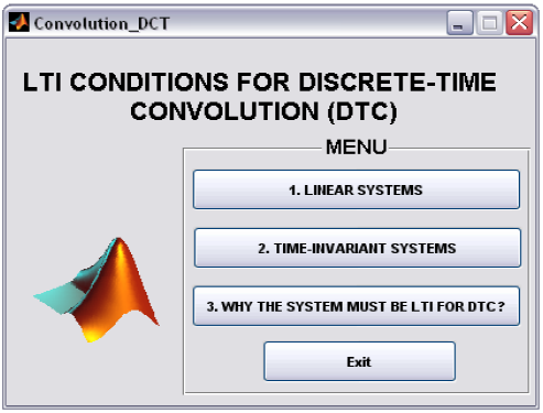
The content of the demo is illustrated in Fig. 2. At the main menu there are three sections, i.e., Linear Systems, Linear Time-Invariant systems, and Why the Systems must be LTI for DTC?
The motivation for the topics in the Menu is many folds:
— To offer a deeper insight into the LTI system characteristics, and
— To provide a better understanding of the convolution operation in the LTI context.
— Provide active participation of students in teaching learning process.
Linear System
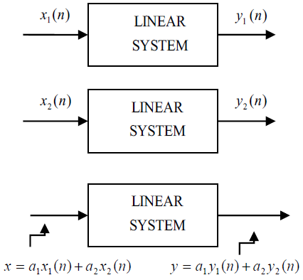
The goal of this demonstration is to visualize the principle of superposition, a property which must be satisfied in linear systems.
In this demonstration it is considered that the linear system is described by its input-output relation:
and two different inputs x1(n) and x2(n) are considered:
as shown in Fig. 3.
In order to assure the active participation of students, they are asked to choose the coefficients of input signals (3, 4) and parameters a1 and a2 from Fig. 3.
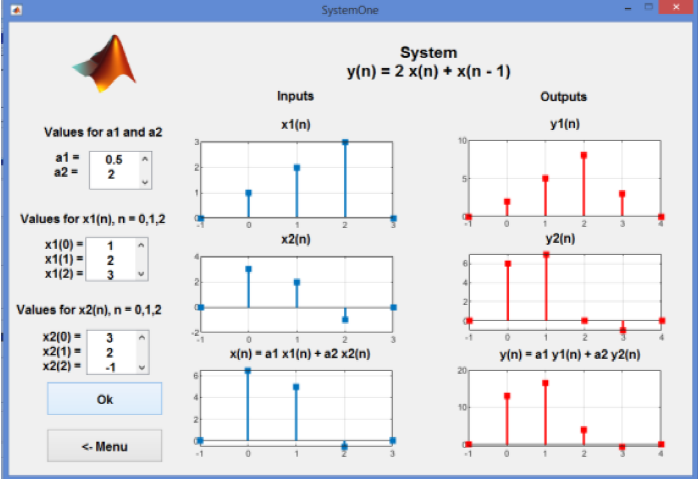
As an example, Fig. 4 illustrates the final slide of this demonstration. On the left hand side, the user gives the values of x1(n) and x2(n) for n = 0, 1, 2, as well as the values of the constants a1 and a2. The plots for xi(n), x2(n) and a1x1(n) + a2x2(n) are shown at the middle of the slide. Finally, the plots on the right hand side illustrate the outputs y(n) and a1y1(n) + a2y2(n). The output y(n) is the response to the inputs x1(n) and x2(n), respectively. Because the outputs are the same, we conclude that the system is Linear System.
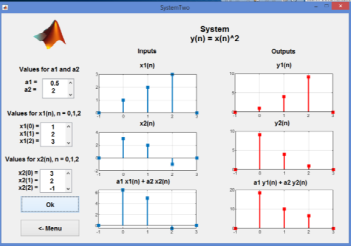
As a second example, consider that the system is given by:
Figure 5 shows the resulting outputs, which confirm that the system is nonlinear.
Time-Invariant systems
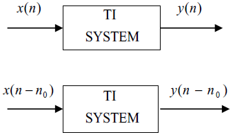
The goal of this demonstration is to show that in the time-invariant systems with the input x(n) and the corresponding output y(n), the shifted input, by n0 samples, x(n-n0) results in the shifted output y(n) by n0 samples, y(n-n0), as illustrated in Fig. 6.
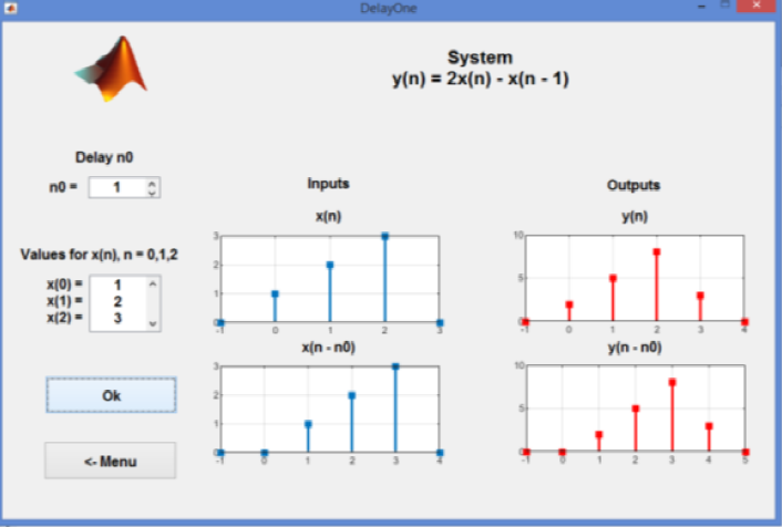
As in Linear System Demonstration Demo, we consider the system given in (2).
Figure 7 illustrates the demonstration results of the demo. On the left hand side, the students choose the values of x(n) for n = 0, 1, 2, and the value of the delay n0. The plots for x(n) and x(n - n0) are shown at the middle of the slide.
Similarly, the plots on the right hand side illustrate the corresponding outputs y(n) and y1(n - n0). The output y(n) is the response to the input x(n - n0), while y(n - n0) is the delayed version of y(n), respectively. From the outputs, we conclude that the system is Time-Invariant System.
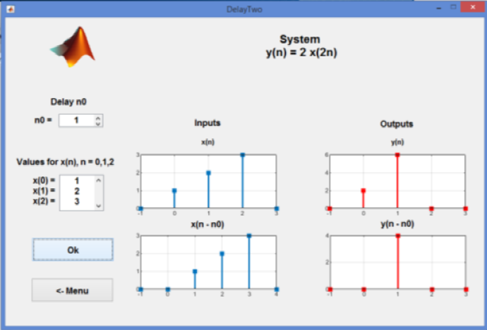
Finally, we consider that the input-output relation of the systems can be written as:
The final slide of the demonstration is shown in Fig. 8, where we notice that the outputs are different. This means that the system is a Time-Variant.
The students are asked to verify if this system is a linear system and thus to demonstrate that a linear system can be a time-variant system.
Why the system must be LTI for DTC?
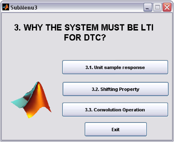
The goal of this demonstration is to show that the conditions of linearity and time invariance must be satisfied in order for the equation (1) to hold. The Submenu of this demo is given in Figure 9.
Unit Sample Response
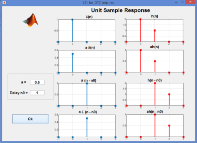
Unit sample response h(n) is a response to a unit sample sequence δ(n):
For a linear system, if the unit sample sequence is weighted by a, x(n) = aδ(n), then the response would be y(n) = ah(n). If the system is a TI system, then the response to a shifted sequence δ(n - n0) is the shifted unit sample response h(n - n0). Finally, if the system is a LTI, then the response to aδ(n - n0) is equal to ah(n - n0).
In this demo, a LTI system is described by the input-output relation given in (2).
The user is asked to choose the value of the parameters a and n0. Figure 10 shows the impulse response, weighted impulse response, shifted impulse response and weighted shifted impulse response for n0 = 1, and a = 0.5.
Shifting Property
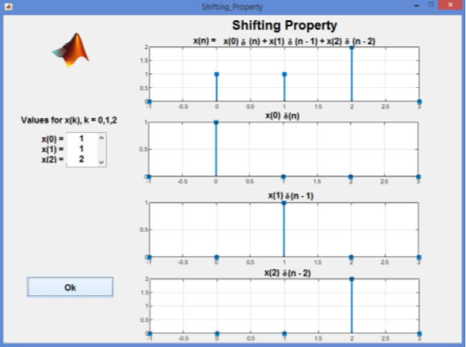
This demo shows that any sequence x(n) can be presented as a sum of weighted shifted unit sample sequences:
User is asked to choose the values x(k) of the sequence (8). Figure 11 illustrates the shifting property for x(0) = x(1) = 1 and x(2) = 2.
Convolution Operation
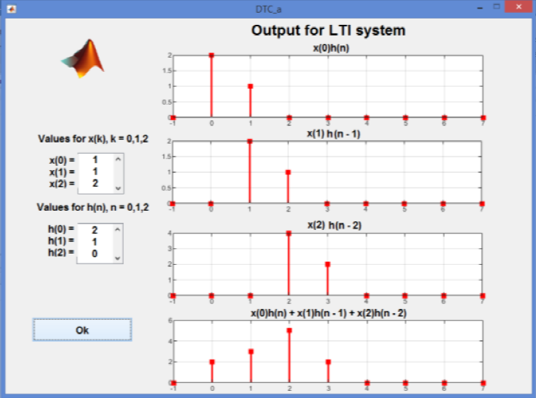
If the system is an LTI, then the response to the scaled delayed unit sample sequence
Is
Figure 12 shows the responses and their sum. Note that the sum of the outputs shown in last row of Fig. 12, presents the convolution, as shown in (1).
Figure 13 presents the input signal x(n) from the first row of Figure 11 and the sum of the outputs (9), shown in the last row of Figure 12:
3 Results and Discussions
First, a theoretical description of the DTC is provided in the classroom. A total of 1.5 hours are used for the theoretical explanations and numerical examples, followed by additional 3 hours for this demo and demo for the computing DT Convolution. Both demo programs are used in two sessions, each lasting 45 minutes.
In the first session the instructor presents the demo programs using a projector. In order to encourage active participation of students during the presentation, the students are asked to propose the demo parameters.
Next session is used for demo program where students run demo on their own laptops using their own parameters. Students are also invited to copy the results of demo in Word document for the followed discussion. After each of 3 demos from Figure 2, there is a discussion about the obtained results. Students compare the obtained results and participate in discussion. Typical discussion topics, for example, are the importance of the superposition principle, the relation of linearity and the time invariance, and the questions such as: can shifting property be applied to any sequence, can we obtain the convolution in a linear time-variant system, can we obtain the convolution in a nonlinear time invariant system.
Students demonstrated very high motivation and actively participated in all steps of demonstrations and discussion.
Students can also use the demo by themselves, after the classes, as an additional tool in solving their homework's.
In order to verify the utility of the demo as a teaching tool a simple 10 minute Quiz is performed before and after this demo presentation and the demo [7]. Additionally, at the end of the course, the same quiz has been incorporated in the overall quiz used to evaluate all demo programs used in the course.
Typical questions for the quiz are the following:
— Q1: Write the expression for the discrete-time convolution (DTC).
— Q2: Present graphically the steps of the DTC for given sequences.
— Q3: What conditions must be satisfied in order to apply the DTC.
— Q4: Explain why the system must be linear in order to apply the DTC.
— Q5: Explain why the system must be time-invariant in order to apply the DTC.
— Q6: Explain why the system must be an LTI to apply the DTC.
The demo presentation has been used for the last five year with a total of 223 students. The Quiz is introduced as a part of the evaluation process, before and after the demo presentation. Correct answers as a percentage of the total number of students (32) are shown in Table 1.
Table 1 Results of Quiz
| Question | Percent of corrected answers before demo presentation |
Percent of corrected answers after demo presentation |
Percent of corrected answers at the end of the course. |
|---|---|---|---|
| Q1 | 100 % | 100 % | 100 % |
| Q2 | 90.625 % | 100% | 100 % |
| Q3 | 59.37 % | 100 % | 100 % |
| Q4 | 6.25 % | 93.75 % | 96.87 % |
| Q5 | 9.37 % | 100 % | 100% |
| Q6 | 6.67% | 90.62 % | 96.87 % |
As expected, the standard questions Q1 and Q2 were largely correctly answered before (and after) the demo presentations. The result demonstrates that after the demo presentations, all students answered correctly questions Q3 and Q5. Additionally, the number of correct answers to the questions Q4 and Q6, increased to 93.75 %, and 90.62 %, respectively, after the demo presentations. Moreover, at the end of the course, when the students are ready for the exam, the number of correct answers additionally improved, as shown in last column of Table 1.
4 Conclusions
This paper presents a new initiative to include a demo program for better understanding one of the most important operation in LTI systems: discrete-time convolution (DTC), and thus complement the demo program for performing DTC operation. The principal motivation to create this demo was to present visually the conditions which must be satisfied in order to apply the DTC.
Therefore, the emphasis was on understanding the fundamental conditions necessary to apply this operation rather than demonstrate the DTC operation. Particularly, we demonstrated why it is necessary that the system must be an LTI (linear-time-invariant) system in order that the DTC can be applied.
This demo has been used as a complement to the theoretical classes in the graduate course Fundamentals of Digital Signal Processing providing the visualization of the topic and the active participation of students in the teaching-learning process. The proposed demo does not need any laboratory equipment and can be applied in the classroom using only a laptop and a projector. Additionally, students can run the programs on their own during and after classes, play with the different parameters, and use the demo as additional help in solving homework. The results of Quiz demonstrated that the demo was an excellent complement in the teaching process and helped students to better understand the concepts of the DTC operation.


 nueva página del texto (beta)


