


 nueva página del texto (beta)
 Inglés (pdf)
 Artículo en XML
 Referencias del artículo
 Enviar artículo por email
 Citado por SciELO
  Similares en
SciELO
Similares en
SciELO 
 Permalink
1 Introduction
Saliency detection in computer vision concentrates on identifying the eloquent and visually dominating region in an image. The objective of salient object detection is to quickly recognize and distinguish the most prominent region in an image just like the human visual system [1]. The human visual system could be imitated technically by the model of visual attention, it is a computational method intended to accomplish the goal of the human visual system, i.e. it involves simulating human eye fixation on a certain area by ignoring other objects.
The salient attention model is used in a wide area of the field like machine intelligence, cognitive psychology, and robotics to increase the effectiveness of visual processing [2]. Its application has not stopped till that, Salient object detection, in contrast is more appropriate for a wide range of computer vision activities [3] including semantic segmentation, object location and detection, content-aware image modification, visual tracking, and human reidentification [4, 5].
It has a wide range of applications because it is more focused on maintaining the integrity of the probable object. Although [6] numerous top-notch models have been released, salient object detection and recognition are still difficult because of a number of intricate elements that are present in everyday circumstances [7].
According to perceptual research [8, 9], the fundamental factor that affects saliency is visual contrast, it’s been effectively proposed in a number of multimodal salient object recognition techniques had built through either global or local contrast modelling [10, 11, 12].
Local contrast models, for instance, can have trouble effectively separating out sizable homogeneous zones inside conspicuous objects, whereas global contrast information may struggle to deal with images with a complex background. Despite the fact that salient object detection is a task for machine learning-based techniques do exist [13, 14, 15], they are mostly focused on merging several saliency maps calculated by various techniques [16].
Deep convolutional neural networks (DCNN) have recently gained popularity in salient object detection due to their potent feature representation, and significantly improved performance over the old techniques [17]. Deep CNN-based techniques inference and training are often carried out region-wise methods, first, a section of an image is split into set of regions or patches.
However, this leads to significant storage and computational redundancies, which require extensive training and testing time, saving the deep features recovered from a single image requires hundreds of megabytes of storage [18]. This limitation motivated us to develop a CNN model using dense computing, and it provides a facility to transfer the input image of any size to a saliency map of the same size. [19] has mentioned several saliency map detection and edge detection using deep learning techniques.
In SOD preserving the outline of the object is so important, it can be attained by simple fully convolutional networks (FCNs), but the result of FCN is mostly a hazy outline because pixel-level correlation is normally not taken into account [20]. So, to learn and to map a complete image to a saliency prediction with pixel-level accuracy, we design a multiscale FCN in the first stream. By extracting visual contrast information from multiscale receptive fields, in addition to learning multiscale feature representations, our FCN can accurately evaluate the saliency of each pixel [21]. The following contributions are made by this paper.
1 To derive a dense saliency prediction straight from the raw input image in a single forward pass, a multiscale VGG-16 [22] network pre-trained for image classification is repurposed as the fully convolutional stream. A grid wise stream has been created in addition to the fully convolutional stream in our network. This stream embosses the saliency discontinuities along region borders, the visual contrast between super pixels, and collects semantic information about important items over multiple layers [23].
2 The performance of saliency detection in object perception is improved by using a multi-task FCNN with a dilated kernel-based technique, which performs a collaborative feature learning process. This also effectively enhances the feature-sharing capabilities of salient object recognition, resulting in a significant reduction in feature redundancy [24]. Using the proposed FCNN model's output, we present a fine-grained super-pixel-driven saliency refinement model.
3 Saliency models like the cutting-edge Amulet, UCG [25] are effective at detecting distracting regions since they typically stand out from their surroundings. This is extremely sensitive to local areas, such as the boundary of a salient item and the local distractions because low-level features are constantly reused. To tackle this issue, we propose a complementary network, called the distraction diagnosis network (DD-Net), which is used to identify distracting regions, lessen their negative effects, and eventually improve model performance [26]. The DD-Net learns to anticipate the distraction score (D-Score) from the input image and produces a noise-free output given to the next level of the model assuring the high-confidence regions. DD-Net decides which areas of a picture should be ignored while saliency detection is being done.
4 Further we build a sparse graph network, where every pixel in this network is connected to both its neighbors and the node that shares a boundary with them has the greatest similarity to those neighbors. The proposed sparse network effectively utilizes the local spatial layout and eliminates unused nodes that distinguish one another one another.
5 Active contour is a technique used in computer vision to detect objects in an image. It is built on the concept of minimizing the energy of the segmentation [27]. The active contour method uses a curve that evolves to fit the boundaries of the object in the image. It does not subject to on the image gradient [28] and can detect objects even when the gradient does not consider object boundaries. The active contour method is used in conjunction with the convex hull technique to accurately detect the salient objects in an image.
To be more precise on the motivation and the contribution of the work, the following briefs it.
| Motivation | Contribution |
| 1) To Handle the Scale Variations in complex background: To investigate the methods for improving the robustness of salient object detection models to variations in object scales and ensuring consistent performance across diverse datasets and scenarios. | To attain the objective [1], VGG 16 architecture been completely remodified according to necessity of our work, especially three were three extra convolution layers (ECL) that are united with the top four pooling layers of the default network, this extra convolution layer performs the dilation operation to gain various scale information from different pooling layers and different dilation rates are used to confirm that no loss salient information occurs. |
| 2) To address Partial Visibility: To explore the techniques to enhance the ability of detection algorithms to localize salient objects accurately, even in the presence of partial visibility, low contrast etc. and improving overall detection performance. | The [2] objective is attained by developing a dense labeling component, which tries to find out the correlation between the two pixels. Equation (1) is formulated to perform the operation, most importantly identifying the appropriate threshold value through several trial been a challenging task and done successfully. |
| 3) To improve the Robustness to image distortions: To develop the techniques to enhance the robustness of detection models to common image distortions, such as blurring, noise, or compression artifacts; ensuring the reliable performance in various imaging conditions. | Objective [3] is one such uniqueness in our work, here the entire distraction detection network (DDNet) is designed for performing the distraction analysis. Formulated the functionality to compute the distraction score of the all the regions, using that the distraction mining is done at ease. |
| 4) To Integrate Semantic and conceptual Understanding: To develop an approach that combine visual saliency with semantic understanding to provide contextually relevant salient object detection, enabling more meaningful interpretations of detected objects within the image. | To have semantic and conceptual understanding of an image, it required to identify the superpixels in every region, and to find the relationship between the superpixels from different region. In our method every superpixel acts as node and the relationship between the nodes acts as an edges and the final graph construction forecast the semantic information that are present in an image. Formulated equation (4), (5) and (6). |
| 5) To optimize salient object detection through energy optimization: To develop a methodology by formulating energy functions that effectively quantify the saliency of objects within images, and incorporating iterative refinement processes to enhance segmentation accuracy by smooth object boundaries. | To obtain a smooth boundary of the salient objects, a network is designed, which computes internal energy and external energy amongst the saliency region to identify the boundary of the objects in an optimal way. Equation (7), (8) and (9) are formulated. |
We evaluate the suggested technique with ten state-of-the-art methods, with six benchmark datasets using a range of evaluation metrics. The results of the testing demonstrate that our strategy performs better than the cutting-edge methods at the moment. The rest of the article is organized as follows.
Earlier research on the dilation algorithm, dense labeling, distraction mining, graph-based salient region detection, and active contour approach is reviewed in Section II. In Section III, we offer the salient region detection method we've recommended. With reference to the datasets for MSRA-B, ECSSD, HKU-IS, DUT-OMRON, PASCAL-S, SOD; which consists of train data, test data and validate data and those test data from the datasets were used for evaluation.
Section IV details the experimental design and results. In Section V, technical details of our framework are discussed, Section VI shows the quantitative comparison and visual comparison of our work with other state of art techniques and in Section VII we conclude the paper.
2 Related Work
The low-contrast image that we receive is to be pre-processed like contrast stretching to enhance the image’s contrast. Fully Convolution Networks consist of multiple convolution layers where these layers apply a set of learnable filters to the input image capturing different features [29]. These filters can help in enhancing the edges and features for low-contrast images. Down-sampling layers like max pooling or stride convolutions help in network focus on capturing larger patterns in low-contrast images.
Skip connections are used in-between layers to preserve low-level features from earlier layers which are particularly valuable in the case of low-contrast images. Alongside Skip connections choosing activation functions is also as important as they will be helpful to introduce nonlinearity and improve the network's ability to capture the relationships between data. [30] uses parametric saliency and non-parametric clustering for saliency detection.
But low contrast images are easily misclassified so choosing an accurate and modified loss function is also important as it helps in semantic segmentation [31]. Different methods involved in extracting information in low-contrast image, histogram equalization, wavelet transform, image fusion, contrast stretching, and deep learning with the dilated kernel are a few.
2.1 Dilation Algorithm
Image segmentation grounded on deep learning has wide applications in autonomous driving, space exploration, the medical field, and in so many other fields [32]. Convolution neural network has a vital role in image segmentation and image classification, but at the same time, it takes too many resources for computation [33]. To address this problem [34] used CNN with a dilated kernel instead of using a convolution kernel, this reduced the training time and improved the accuracy of their model.
But in contrast, hybrid dilated CNN was built by stacking DCNN with different dilation rates on the kernel and still got further improvement in the accuracy of image classification. Deeplab framework [35] uses multi-scale neural networks using sparse convolution, their dilated network is used for feature extraction, and it focuses on high-level and low-level features to obtain highly accurate segmentation results.
The dilation filter [36] has a strong impact on edge detection algorithms to obtain accurate edge map results. The most difficult task of segmentation is performing it on low-contrast images, [37] uses morphological transformation for background approximation and has the conjunction of multiple background analyses.
In an application of classifying hyperspectral images [38] used MDCNN. This framework helps to reduce the complexity, efficiently concatenates every hyperspectral information in the map, and generates the feature map with a limited number of parameters.
Fig. 1 shows the reference diagram of using dilated kernel to classify an image, it mentions the necessity of using dilation kernel, in general using of Convolution neural network has a vital role in image segmentation and image classification, but at the same time, it takes too many resources for computation. To address this problem [39] used CNN with a dilated kernel instead of using a convolution kernel, this reduced the training time and improved the accuracy of their model.
2.2 Dense Labeling
Dense labeling is a simple, faster, and efficient way of processing the saliency and its important concept is extracting knowledge from low-contrast images. [40] performs saliency estimation on macro objects and approximates the location of the object as well. In this regard [41] uses super pixel values to estimate the dense depth information in an image.
This framework has been designed with the idea of being generic in addressing all types of images. Dense labeling along with DCNN and SVM is formulated in for multiclass semantic segmentation. SVM explores different representations of multi-class objects which are indirectly related to identifying the target object and it is combined with DCNN for efficiently segmenting the respective class objects. Semantic segmentation is used not only for static images but also in addition for real-time images.
It employs an innovative approach to dealt with the images captured by multiple cameras, here the issue is information on the image is captured by only a few viewpoints, and the rest nullifies the output. So functional color-based labeling method is incorporated to attain the desired output [42].
For evaluation remote sensing image retrieval used the dense labeling concept, especially for the dataset that contains multi-classes. RSIR used features-based extraction with deep learning techniques for more efficient performance.
2.2.1 Distraction Mining
In general, any segmentation process suffers from false positive or false negative values that distract the objective of the work [43]. So, the latest research on segmentation has a foresight on distraction identification, which focus on categorizing the noisy data that are merge with target objects and reduces the accuracy [44]. The COS framework concentrated on the focus module to remove the distractive noisy background that is alike to the target object.
It estimates the distraction and its position for removal, through this the segmentation of the target object is made perfectly.
In medical image processing minimizing false ratio is one the most desirable outcomes, in spite of that DSNet [45] uses two models namely the neighbor fusion model to concatenate high-level features and the distraction separation model aims to catch object information by ignoring the distraction [46].
2.2.2 Graph Construction
Graph-based segmentation has attained more popularity in recent years [47]. The graph-based approach divides the image as a graph of multiple subgraphs, each representing the expressive region of the image.
PSA [48] recognizes the indirect impact of background on the eloquent region through the graph to get accurate output. GBA generates a set of weights for the nodes and connectivity among the nodes to create the target image content.
Using Eigenvalues and covariance values [49] computes the weightage of the nodes for segmentation. The DWCut works efficiently with fewer number parameters also.
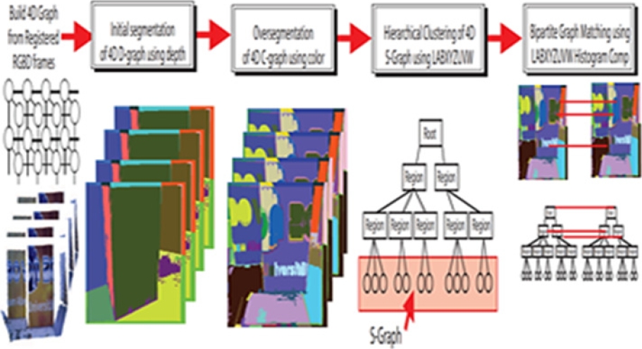
Fig. 2 describes about graph construction based on hierarchical clustering technique.
3 Proposed Methodology
Fig. 3 shows the framework of the proposed work, where the raw input image is passed over fully convolutional neural network for feature extraction and the dilation kernel with different kernel rate are convolved over the image to extract the feature with scale variance, saliency map along with probability value is generated as output and it is processed through dense labeling (DL) and distraction mining (DM) component.
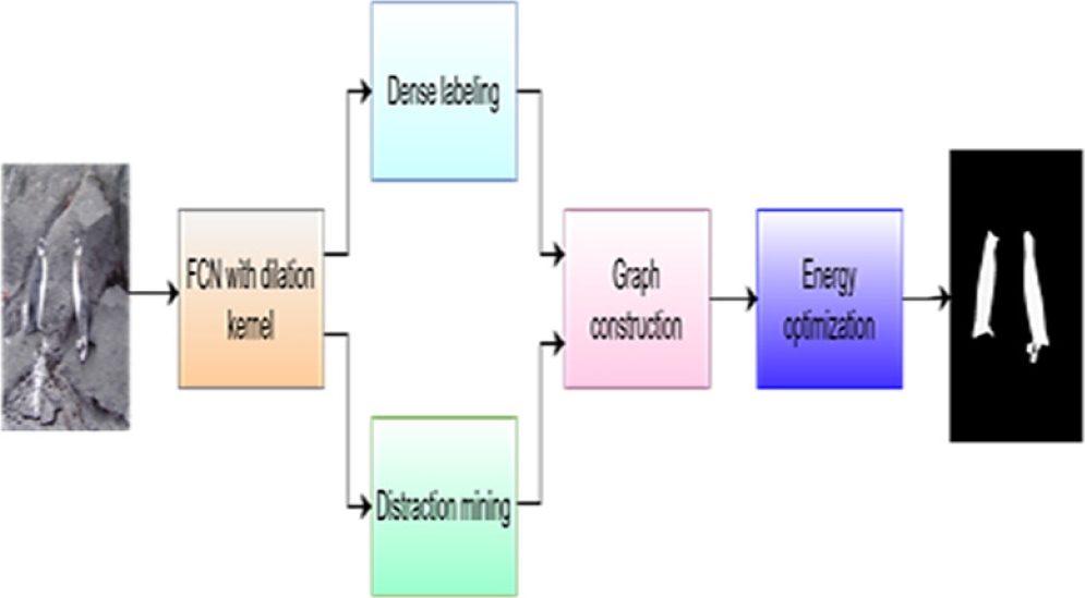
DL segregates the foreground and background pixels based on the relationship between the pixels and DM is one which identifies the pixel region that were redirecting the detection process.
Further the output of DL and DM is processed and the graph is constructed based on the super pixel values and finally the energy optimization function brings out the smooth salient foreground image as an output [50].
Pseudocode of our Framework
1 Load the image and pass it through a fully convolutional neural network (FCN) for feature extraction.
2 Convolve the dilation kernel with different kernel rates over the image to extract features with scale variance and generate a saliency map along with probability values as output.
3 Process the saliency map output through dense labeling (DL) and distraction mining (DM) components.
4 DL: Segregate foreground and background pixels based on pixel relationships.
5 DM: Identify pixel regions that redirects the detection process.
6 Process the output of DL and DM, construct a graph based on the super pixel values.
7 Optimize energy function to obtain smooth salient foreground image as output.
8 Compute external and internal energy terms.
9 External energy: Combine data term and smoothness term using optimization technique.
10 Internal energy: Define constraints or penalties to enforce desired properties of the contour.
11 5.2. Obtain the saliency map.
3.1 Fully Convolutional Networks with Dilation Kernel (FCNDK)
FCN focus on understanding images at the pixel level and creating a comprehensive pixel-by-pixel regression network.
This network transforms the raw input image into a detailed saliency. By considering the vitality of contrast modeling and the size of objects in saliency detection, we consider the following issues into consideration when designing the structure of our FC network. On account to identify visual saliency, which always depends on low-level characteristics and high-level features for contrast modeling, the network should be significant enough to include multi-level information at the outset.
The FCN should then be able to project the object at different sizes, which is why scale-aware contrast modeling is also a priority. Lastly Training the images through every pixel is a necessary and extremely important task for accurate detection, for convenience, rather than starting the training for the model from scratch, we preferred to use a pre-existing network for simplicity.
One such kind of the most adopted and publicly accessible pre-trained model is VGG-16. However, for obtaining the output as per our requirement few modifications are incorporated on the default model of VGG-16, firstly the down sampling rate [51] is reduced by using the stride of 1 instead of 2, through which high-resolution saliency is obtained. Generally, FCN is accurate for making any prediction nevertheless, there are few limitations for FCN for segmentation, i.e., individual pixel contexts should be preserved for accurate pixel prediction.
It could be compensated by using dilation convolution in FCN. The advantage of using dilation convolution in FCN is, that it increases the attentive field of the convolution layer excluding extra parameters and as well which does not increase the computational complexity.
In FCN using pooling and strides sometimes reduces the spatial information of an image, whereas with the help of dilation convolution, more spatial pieces of information are preserved which is more vital for the segmentation process. Finally, by varying the dilation rate across the FCN, the model can adapt to gain knowledge on different patterns with different scales.
Therefore, using dilation convolution in FCN leads to improved performance of the model and is thus incorporated here. A framework like Caffee has built-in dilation convolution to efficiently control all these mentioned operations. Moreover, dilation convolution enables us to manage the density of the features in our designed FCN. Here is a comprehensive explanation of the working of VGG-16 in our model. VGG-16 have five max pooling layers (PL), which takes the input image and could able to create a large receptive field with more contextual information.
Additionally, it becomes complicated to process further rapidly and also increases the computational timing. So as a key three extra convolution layers (ECL) are united with the top four pooling layers, this extra convolution layer performs the dilation operation to gain various scale information from different pooling layers without losing any salient information.
The ECL down samples the pooling output to an equal-sized receptive field with the strides of 4,2,1,1 respectively. These four ECL outputs are unified with five PL outputs and a single output is generated, to which a sigmoid activation function is applied to acquire the probability of the saliency map.
3.2 Dense Labeling
Dense labeling is the process of separating the foreground object and background object in an image. The FCN has produced the salient probability map, which is further processed to segregate the foreground and background. Using the correlation heat map (CRHM) those pixels are processed to be represented in graphical form with different colors, which makes it simple to visualize the information and make the picture clear and accessible [52].
The idea is to take the saliency probability map values and plot color codes based on their values on the grid. The higher gradient (foreground region) is often represented with warmer colors and the lower gradients (background region) are represented with cooler colors.
The correlation coefficient is computed for the pair of probability maps. Two variances of correlation may arise, a positive correlation in which one feature tends to increase another one, and a negative correlation tends to decrease the other features. Heatmap (hmap) is generated based on the pair of values where positive represents the warmer color and negative uses the cooler color.
The equation for positive and negative correlation are as follows:
where,
Cov(m,n) represents the covariance between the two variables X and Y.
E denotes the expectation values of the terms that follows.
m - µXm & n - µn are the deviations of X and Y from their respective means µXm & µn.
µXm & µn are the means of X and Y respectively.
σm * σn are the standard deviations of X & Y respectively.
The resultant heatmap [53] is the graphical image of the correlation of the features, which helps in getting accurate segmentation in further progress.
3.3 Distraction Mining
Major issues with saliency detection are distracting the process with undesired regions, i.e. Which is not a region of interest (ROI). Distraction mining is a process used to identify distracting regions in an input image that can negatively affect the performance of a saliency detection model. The analysis is performed by a Distraction Detection Network (DD-Net), by predicting each pixel’s probability value that is distracting. The DD-Net is trained using a distraction mining method, which simulates the absence of specific regions and evaluates the changes in saliency prediction.
Regions that cause negative prediction changes are considered distracting patterns and are used to train the D-Net. The analysis helps improve the performance of the saliency detection model by identifying and minimizing the negative effects of distracting regions. To lighten the unwanted sensibility and to attain better results we use a learnable network to detect the distraction that degrades the efficiency of the process.
The idea follows by mining the distraction from the input and then training the network to avoid the distraction. But in which way the mining is done, is the biggest problem; because doing more advanced calculations is not appropriate for mining the distraction from the input.
So, in our proposed work, we use the threshold values (TV) to accomplish the goal. All the actual values are in the form of binary images which represent saliency value as 1 and non-saliency as 0 and this is considered as a tweeting point.
As from the previous process ie. via FCN, a saliency probability map is already obtained, the probability map with a threshold value 0.6 and above is well thought of as a foreground region, and the region lesser than that is frozen as a background object, i.e., treated as a distraction. The forthright way of doing this is applying global thresholding, where the TV is chosen and for every saliency probability map, this threshold is applied and classified as foreground and background which is mentioned as a coarse grain saliency map (cmap). Equation:
A coarse grain saliency map creates the saliency in a new dimension. The higher threshold pixel is determined in the previous step, through traversal of the salience pixel along with the four nearest pixels is performed with an elementwise product operator, and a new dimension is computed:
where, P(i,j) is pixel value with spatial coordinate i & j.
3.4 Graph Construction & Weighting
The hmap and cmap are diffused together to give the details of the feature in the image. These features represent the content of the image which includes intensity, and other low-level visual characteristics. The idea of a diffused saliency map is to highlight the salient regions and to suppress the background region.
Later the highlighted region is normalized to ensure the score lies in the region of 0 and 1 for better conception. In general, the spatial region of a salient object is lesser than the area of the background in an image [54], it motivates to the computation of the saliency seed for background and foreground separately and to construct the graph based on their similarities.
The complete image is split into two clusters, i.e., as foreground and background the process is further progressed. Clusters are denoted by a radius, the pixel at the centroid of the radius is picked as seed, and the surrounding pixels around it is well thought of as neighbor pixels which are taken into consideration for similarity measure.
It compares the intensity of the center pixel with the neighbor pixel, if it outputs a higher value than or equal to the center pixel, that pixel is treated as a salient pixel, and a graph is constructed. The same procedure is followed for background cluster spatial areas also. The outcome of this process is going to be a super pixel feature vector of salient objects.
So far, a regular graph is constructed with super pixels and the weight of the super pixels is calculated for the saliency values of nodes. Weighing the super pixel is important because it becomes unreliable when the seed nodes are mixed with noises which it produces undesirable results and also fails to identify the salient objects. However, weighing the super pixels prominent the visuality. The further improvement of the salient feature is done by:
where,
S(x) is saliency value of foreground superpixel.
b(x,y) is normalized weight for a(x,y).
a(x,y) is weight of saliency value.
3.5 Energy Optimization
The last step is to attain the saliency confidence map and cut the edge of the boundaries of the object through the energy optimization (EO) concept. The working of EO completely relies upon the probabilistic value of the weighing pixel which was obtained using the graph-based weighing method and as a result, each pixel represents as if it belongs to the foreground or the background.
Usually, the traditional method works on the intensity cue but the EO generated the confident map of SO by contouring from the high probability values towards the boundaries and is treated as external energy of the saliency map. EO iteratively updates the shape of the saliency by moving laterally in a way that decreases the energy until it converges the object boundaries of the salient object.
The iteration process determines the optimal position that is incorporated in the objects. Meanwhile, the internal energy is also in charge of regulating the contour's regularity and smoothness from not differentiating out of the desired shape.
The values that are out of the external energy are taken as the background and not contoured. The optimal energy of saliency is given by:
where,
Eexternal is calculated upon the data term and Einternal is calculated using smoothness term.
data term represents the value of the super pixel feature Fij and Sij of the reference value and saliency value respectively at pixel(i,j).
Doing the above steps overcomes the problem of dealing with low-contrast images and also with complex images [55]. The iteration process plays a significant role in minimizing the total energy that an object possesses which leads to an accurate saliency map.
3.6 Salient Object Recognition - Saliency Map
Salient object recognition or saliency detection does not mean labeling the image, it focuses on grasping the intention of visually attentive objects, Saliency recognition deals with which part of the image has the salient object [56]. For labeling the detected object labeling methods can be used. The final output of the framework is a saliency map.
4 Experimental Results
The proposed work uses the six most widely used datasets [57] for evaluation purposes, the MSRA-B dataset used to facilitate the evaluation and development of algorithms for identifying salient regions in images.
It has 5000 images in the dataset that cover outdoor scenes, indoor scenes, natural objects, man-made objects, and many more along with ground-truth saliency maps which makes evaluation easier; moreover, due to the complexity and diversity of the images, it makes the model robust for saliency detection.
SOD [58] dataset has more than 5000 images with corresponding ground truth saliency maps. This dataset includes multiple objects with low contrast, which is again a challenging task for saliency detection.
Datasets from were referred, ECSSD, HKU-IS [58] which is from the previous work that contains complex scenes with challenging backgrounds and cluttered images. DUT from previous work, this dataset contains various levels of complexity and has 5168 challenging images, which have relatively complex and diversified contents. PASCAL from previous work and contains 850 natural images.
4.1 Evaluation Criteria
The evaluation metrics like Precision-Recall, F-measure and mean absolute error were used to assess the effectiveness of our model on salient object detection [59].
a) Precision provides positive prediction value ie. which says about true positive prediction value to how many were actually positive. The higher precision value indicates the model prediction positive outcome which is considered to be correct. Significantly false positive leads to crucial consequences:
b) Recall speaks about the correct positive rate, i.e., the measure of the proposed work on the ability to properly identify all the positive instances. In detail it says about among all actual positive instances, how many the model predicted correctly. An increased recall value suggests that the model predicts all positive values correctly. Increasing the threshold increases the precision and decreases the recall rate and vice versa. It is so important to choose the appropriate threshold to determine the model effectiveness:
c) F-measure [60] gives the harmonic mean of precision and recall, it considers both false positives and false negatives, which provide a single balanced value of both:
d) MAE stands for mean absolute error, which is the average error between the saliency map and the ground truth on a per-pixel basis. MAE provides a direct way to evaluate or to compare the model-predicted output with true values:
5 Technical Details of Our Framework
For training the model with different datasets, GPU with RAM size of 32GB, along with 500GB HDD and PCIe 4.0 for high-speed SSDs is used. Linux operating system, Python 3.11 version with the framework like TensorFlow, PyTorch, Keras etc. been utilized.
5.1 FCNDK
For the training process all the images are resized to 320x320. The training is performed using the VGG-16 and is trained with a learning rate of 10-3. The weight decay [61] is provided as 0.0005, with momentum of 0.9 on training.
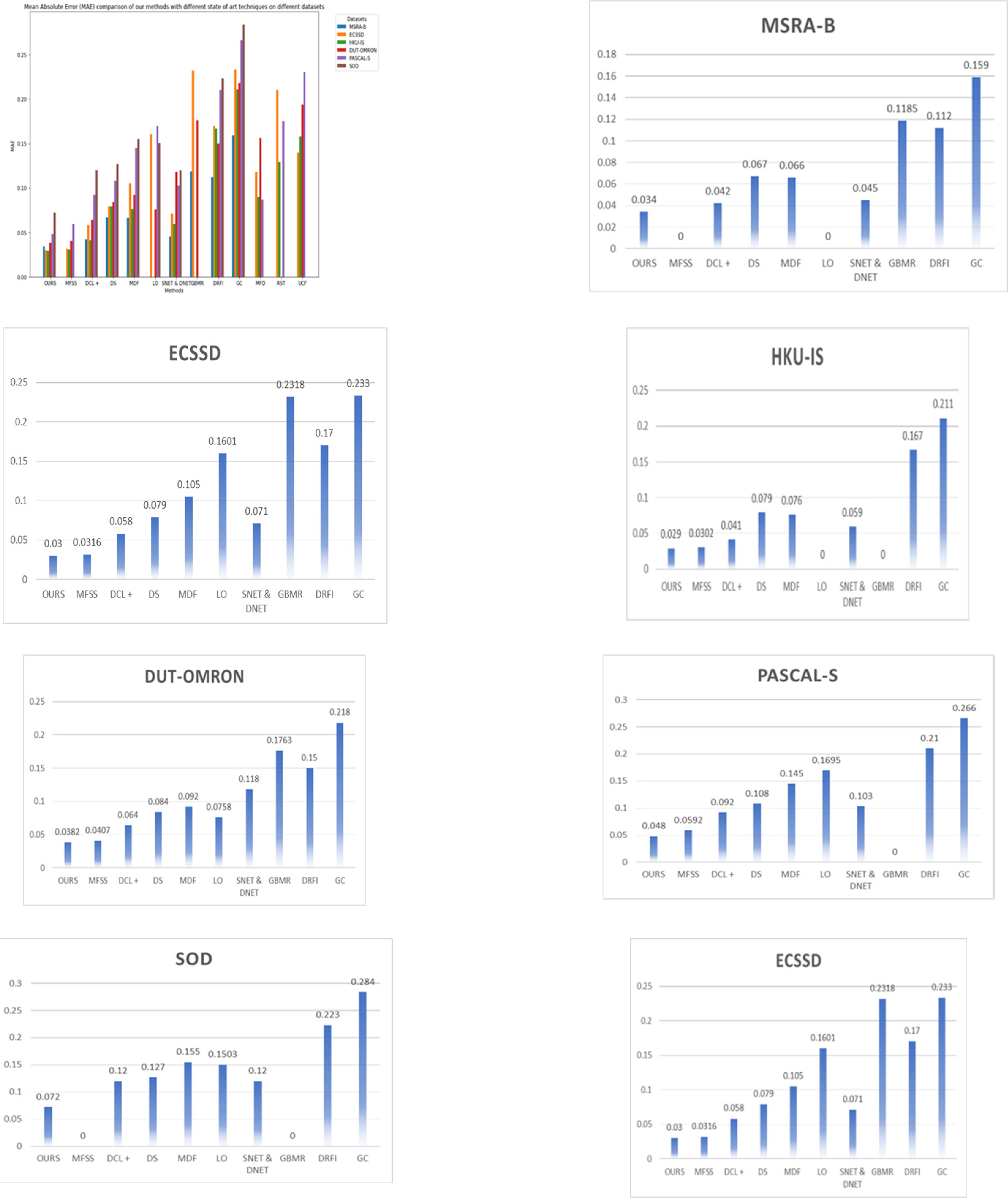
Table 1 Quantitative evaluation results of GSD framework against ten state-of-the-art conventional saliency detection methods
| Datasets | Criterion | OURS | MFSS | DCL+ | DS | MDF | LO | SNET & DNET | GBMR | DRFI | GC |
| MSRA-B | F- Measure | 0.942 | - | 0.931 | 0.898 | 0.885 | - | 0.923 | 0.8562 | 0.845 | 0.719 |
| MAE | 0.034 | - | 0.042 | 0.067 | 0.066 | - | 0.045 | 0.1185 | 0.112 | 0.159 | |
| ECSSD | F- Measure | 0.939 | 0.9341 | 0.925 | 0.9 | 0.832 | 0.8095 | 0.917 | 0.6617 | 0.782 | 0.597 |
| MAE | 0.03 | 0.0316 | 0.058 | 0.079 | 0.105 | 0.1601 | 0.071 | 0.2318 | 0.17 | 0.233 | |
| HKU-IS | F- Measure | 0.947 | 0.9305 | 0.913 | 0.866 | 0.861 | - | 0.922 | - | 0.776 | 0.588 |
| MAE | 0.029 | 0.0302 | 0.041 | 0.079 | 0.076 | - | 0.059 | - | 0.167 | 0.211 | |
| DUTOMRON | F- Measure | 0.917 | 0.872 | 0.811 | 0.773 | 0.694 | 0.7449 | 0.77 | 0.5631 | 0.664 | 0.495 |
| MAE | 0.0382 | 0.0407 | 0.064 | 0.084 | 0.092 | 0.0758 | 0.118 | 0.1763 | 0.15 | 0.218 | |
| PASCALS | F- Measure | 0.922 | 0.901 | 0.857 | 0.834 | 0.764 | 0.818 | 0.845 | - | 0.69 | 0.539 |
| MAE | 0.048 | 0.0592 | 0.092 | 0.108 | 0.145 | 0.1695 | 0.103 | - | 0.21 | 0.266 | |
| SOD | F- Measure | 0.873 | - | 0.848 | 0.829 | 0.785 | 0.7807 | 0.853 | - | 0.699 | 0.526 |
| MAE | 0.072 | - | 0.12 | 0.127 | 0.155 | 0.1503 | 0.12 | - | 0.223 | 0.284 |
5.2 Dense Labeling
The dense labeling (DL) step in our work aims to predict a complete label mask to each of the pixel [62] of the input image. It uses a deep neural network (DNN) to conduct DL that directly outputs an initial saliency estimation for the given input image. The DL network is trained using a training dataset and it is designated to maximize the preservation of global image information and provide accurate location estimation of the salient object. The DL network architecture comprises of numerous layers including fully connected, pooling, and convolutional layers. The DL network takes the FCNDK output as input and produces a Heatmap as output.
5.3 Distraction Mining
The Distraction Detection [63] Network (DD-Net) is one of the components in proposed model for detecting salient objects. It is designed to identify and minimize the negative effect of distracting regions in an input image.
The DD-Net learns to predict the distraction score for each location in the image. The distraction mining approach computes a distraction score for each location in the image using a sliding window.
The regions with high distraction scores are considered distracting and are masked out in the input image [64]. The modified image, with distracting regions removed, is then fed to the further process for saliency prediction. The DD-Net is trained with a mini-batch size of 10 for 20 epochs. The distraction mining is performed on a given image by computing the distraction score with a 20x20 pixel sliding window and stride with 2 pixels [65] are scanned through the entire image.
Overall, the DD-Net component reduces the negative influence and enhances the framework's performance by foreseeing the distracting regions on saliency prediction. It helps the model to concentrate on the salient object and produce better saliency predictions. It is implemented using the publicly available Caffe library. For the DD-Net, it is trained using a mini-batch size of 10 for 20 epochs, with a learning rate of 5×10⁻⁹. The outcome of the DD-Net is the distraction score for each location for the provided input.
This score indicates the likelihood of a particular region being distracting and negatively influencing the saliency prediction.
5.4 Graph Construction and Clustering
Generating the graph involves connecting each node to neighboring nodes [66] and the most similar node sharing a common boundary with the node next to it. Additionally, nodes on the four edges of the image are interconnected to reduce the geodesic distance between similar super pixels.
This sparse graph effectively uses the spatial relationship and removes dissimilar redundant nodes, ensuring better performance. The weight of each edge is determined based on the Euclidean distance between the mean Lab color features of the corresponding super pixels.
For constructing the graph, the proposed work encompassing three components: graph construction, robust sparse representation model with weights and saliency measure. An undirected regular graph with super pixels as nodes is created during the graph creation phase.
A local neighbourhood spatial consistency is taken into account when connecting each node to its nearby neighbours. The background seed nodes are chosen to be the image boundary nodes. The weight of the edges is distinctly created on the spatial distance between nodes. nodes on the four edges of the image are associated to each other.
This sparse graph effectively utilizes the regional spatial relationship and removes dissimilar redundant nodes. Overall, the graph construction for salient region detection involves connecting nodes based on spatial relationships and similarity, resulting in improved performance of saliency detection.
The resulting graph represents the super pixels and their relationships. The best representation coefficients are determined once the graph has been created and reconstruction errors are computed for each super pixel. This is done by solving an optimization model that minimizes the sparsity of the representation coefficients and the reconstruction errors. Iteratively updating both the reconstruction errors matrix and the representation coefficients matrix is the solution until convergence is reached.
5.5 Energy Optimization
In the proposed model, energy optimization has a vital role on detecting salient objects [67]. The energy values are regularized in the range of 0 and 1. The higher energy value of a pixel, the more likely it is to become a key point. The energy optimization process involves minimizing the energy function with respect to certain constants, which are expressed as functions of the active contour. The iterative model updates the active contour by the convex hull formed by the key points.
6 Output Comparison
6.1 Quantitative Details of the Proposed Method
The below table shows the performance of the proposed work. For fair comparisons with other models, we use the implementation results with recommended parameters and the saliency maps provided by the authors.
The quantitative evaluation result of our model along with existing cutting edges techniques are plotted as Precision Recall (PR) curve and MAE graph. The existing methods experimental values are used as such from the reference papers for the comparison.
From Fig. 4 the PR curve of our GSD model performs well in terms of F-measure, GSD PR curve is higher than all comparison methods.
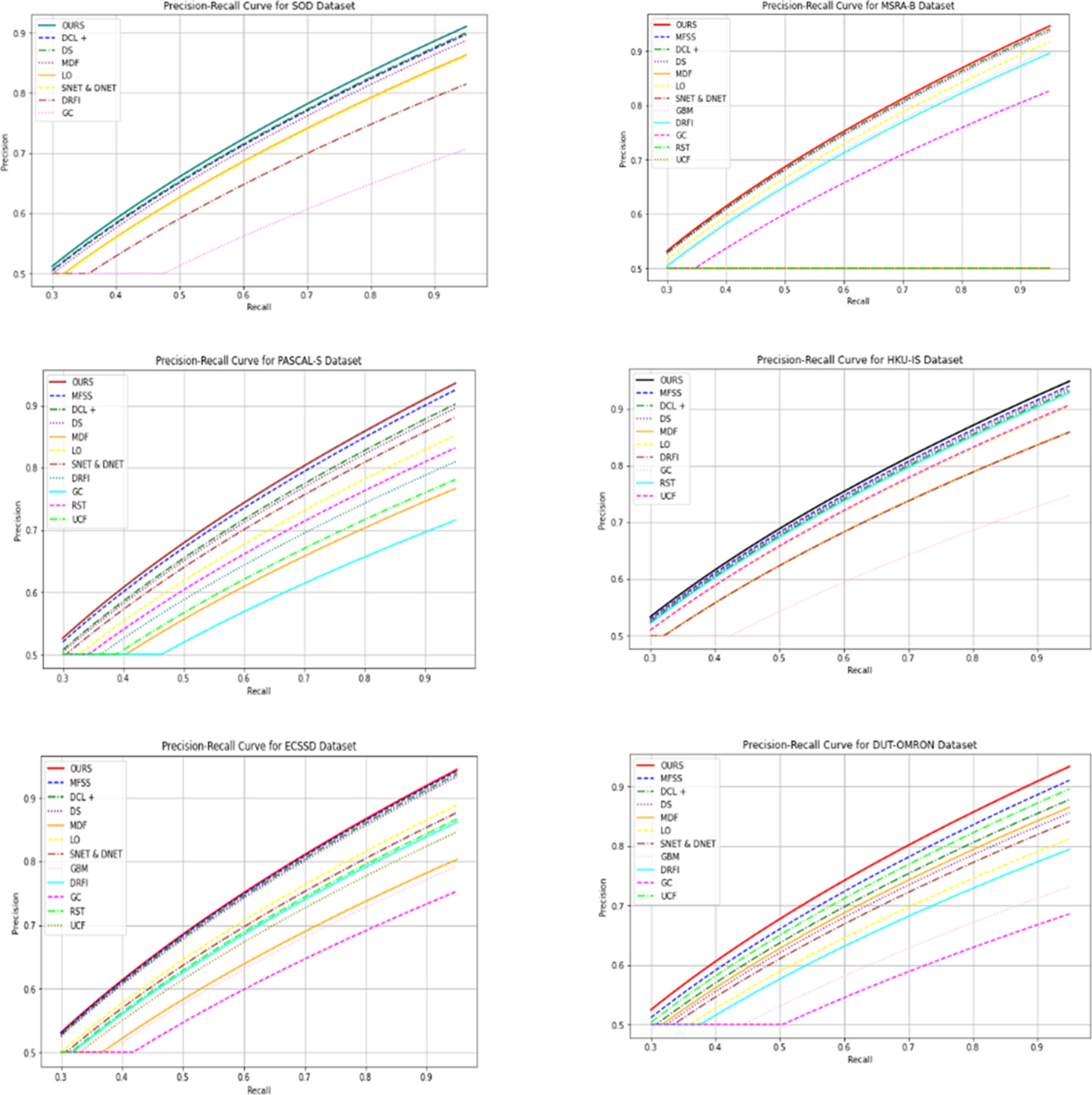
Fig. 5. shows the mean absolute error is comparatively lesser than all other models. In the below graph MAE values is taken and compared our framework with other state of art techniques.
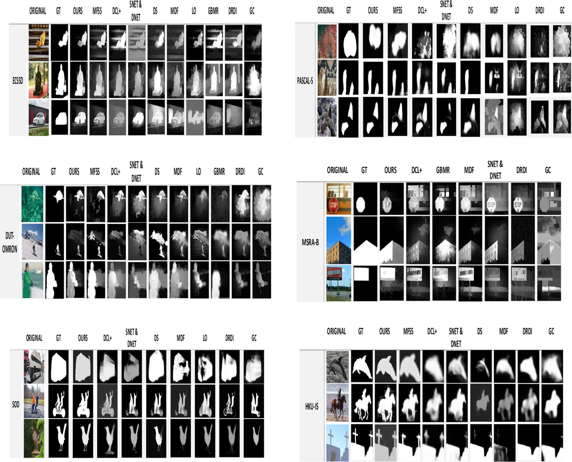
6.2 Visual Comparison
The visual comparison result shows the comparison of our framework with cutting-edge techniques. In the visual comparison it is clearly visible that our model performs better than the existing models. To forecast the performance of our proposed model the images with low contrast, complex background and highly interfering background are considered for evaluation, and our model out performs for all the types of images while comparing with the existing state of art methods and the visual comparison proves that.
7 Conclusion
The suggested strategy is anticipated to perform better than current techniques in terms of accurately detecting salient objects, particularly in difficult situations with distractions and intricate backgrounds.
The accurateness and dynamicity of saliency detection are expected to be improved by the addition of multi-level features, dense labeling, distraction analysis, graph construction, and active contour refining.
In computer vision applications, the combination of these techniques is anticipated to increase the object recognition and scene comprehension accuracy and robustness of saliency detection. The efficiency of the suggested strategy is confirmed by the experimental findings and comparisons with current approaches.
Moreover, in proposed work, the majority of the challenges that exists in salient object detection and recognition is addressed, nevertheless, the framework could further focus on handling the low-resolution images without involving too much complex functionality and to do the recognition with a mean time. This could be the one of the future works that can be augmented in our framework.

