Artículos
Control and signal filtering system for a quadcopter; analysis, comparison and implementation via low-cost IMU and microcontroller
Sistema de control y filtrado de señales para un quadrotor; análisis, comparación e implementación mediante IMU de bajo costo y microcontrolador
Allende-Peña, Jacobo Marcos1
 http://orcid.org/0000-0003-1227-0449
Rodríguez-Paredes, Salvador Antonio2
http://orcid.org/0000-0002-1725-9874
Salmerón-Quiroz, Bernardino Benito3
http://orcid.org/0000-0001-9028-8287
http://orcid.org/0000-0003-1227-0449Rodríguez-Paredes, Salvador Antonio2
http://orcid.org/0000-0002-1725-9874Salmerón-Quiroz, Bernardino Benito3
http://orcid.org/0000-0001-9028-8287
-
Publication dates-
July 30, 2021
Apr-Jun , 2021
- Article in PDF
- Article in XML
- Automatic translation
- Send this article by e-mail
- Share this article +
Abstract
This work presents the development, analysis and comparison of dynamic models, to implement in a simple way a filtering and control system for a quadcopter through the use of a microcontroller. A non-linear dynamic model obtained from the Euler Lagrange equations is approached; also a simplified non-linear model from the first model and a linear model are obtained. Subsequently, making use of each model, controllers are designed using the computed torque controller technique, then, their performance index is obtained through numerical simulations applied to the complete non-linear model to compare their response. Afterward, with the various models and through observers and Kalman filters, signal filtering systems are synthesized for a low-cost Inertial Measurement Unit (IMU), the filtering results are also compared using a performance index. Additionally, the proposed controller is compared in simulation with a fuzzy logic controller. Finally, the selection of the model, the controller and filtering are validated through experimentation with a quadcopter prototype developed by the authors, based on an experimental platform with four rotors, a fiberglass structure, a microcontroller and an IMU MPU 6050.
Keywords::
Quadcopter, model analysis, computed torque controller, Kalman filter, observer, low-cost IMU, implementation, microcontroller
Introduction
In recent years, the rise of unmanned aerial vehicles (UAV) has had a great impact on society so the area of possible applications increases continuously, for example: in the field of the military, trade, the search, rescue, dangerous environment monitoring, product delivery, as well as others (Floreano & Wood, 2015; Gupta et al., 2013; Cárdenas, 2015; Gutiérrez et al., 2017.
-
Floreano & Wood, 2015Science, technology and the future of small autonomous dronesNature, 2015
-
Gupta
et al., 2013Review of unmanned aircraft system (UAS)International Journal of Advanced Research in Computer Engineering & Technology (IJARCET), 2013
-
Cárdenas, 2015Drones Ciencia al Vuelo¿Cómo vez?, 2015
-
Gutiérrez et
al., 2017El uso de drones en ciencias de la tierra, 2017
One of the main problems, when is generating a control system for an aerial vehicle, is to develop a dynamic model that describes the real behavior of the aircraft in the most precise way possible and at the same time; keep the model simple to design, analyze and investigate various control strategies, signal filtering, as well as implement the controller and filtering system in a digital system in a simple way. The quadcopter mathematical model is a set of equations that allows representing in detail the dynamic behavior of the quadcopter in flight; one of the main ways to approximate the dynamic model is applying the Euler-Lagrange methodology, which consists in observing the angular velocities of the vehicle, from a reference frame, movable but aligned to an inertial frame (Sadr et al., 2014; Rodríguez et al., 2016; Balasubramanian & Vasantharaj, 2013; Nonami et al., 2010; Beard & McLain, 2012; Garcia et al., 2006; Castillo et al., 2007; Carrillo et al., 2012; Raffo, 2007), this methodology incorporates the inertial and gyroscopic effects of the aircraft structure into the model. On the other hand, there is a model developed using Newton-Euler, which observes the angular velocities of the quadrotor from a mobile frame defined in the center of rotation of the aircraft (Bouabdallah & Siegwart, 2007; Falconi & Melchiorri, 2012; Elruby et al., 2012; de Jesus Rubio et al., 2014; Paiva, 2016; Bouabdallah & Siegwart, 2004; Hossain et al., 2010; Patete & Erazo, 2016; Agho, 2017), in this model, it is common to observe that the gyroscopic and inertial effects of the aircraft structure are despised, however, the gyroscopic effect of the rotation of the propellers is incorporated. Also, there are linear approximations, in which the flight dynamics around an operating point are frequently approximated (Sabatino, 2015; Roldan, 2016; Sevilla, 2014).
-
Sadr
et al., 2014Dynamics modeling and control of a quadrotor with swing loadJournal of Robotics, 2014
-
Rodríguez et al., 2016Comparación de modelos matemáticos y controladores PID vs LQR para un cuadricóptero, 2016
-
Balasubramanian & Vasantharaj, 2013Dynamic modeling and control of quadrotorInternational Journal of Engineering and Technology (IJET), 2013
-
Nonami et al., 2010Introduction. In Autonomous Flying Robots, 2010
-
Beard & McLain, 2012Small unmanned aircraft: Theory and practice, 2012
-
Garcia
et al., 2006Modelling and control of mini-flying machines, 2006
-
Castillo et al., 2007Modelado y estabilización de un helicóptero con cuatro rotoresRevista Iberoamericana de Automática e Informática Industrial RIAI, 2007
-
Carrillo et al., 2012Quad rotorcraft control: vision-based hovering and navigation, 2012
-
Raffo, 2007Modelado y Control de un Helicóptero Quad-Rotor, 2007
-
Falconi &
Melchiorri, 2012Dynamic model and control of an over-actuated quadrotor uavIFAC Proceedings, 2012
-
Elruby et
al., 2012Dynamic and control of quadrotor vehicleThe International Conference on Applied Mechanics and Mechanical Engineering, 2012
-
de Jesus Rubio
et al., 2014Comparison of two quadrotor dynamic modelsIEEE Latin America Transactions, 2014
-
Paiva,
2016Modelado y control de un cuadricóptero, 2016
-
Bouabdallah & Siegwart,
2004PID vs LQ control techniques applied to an indoor micro quadrotorIEEE/RSJ International Conference on Intelligent Robots and Systems (IROS)(IEEE Cat. No. 04CH37566), 2004
-
Hossain et al.,
2010Bond graph dynamic modeling and stabilization of a quadrotor helicopterResearchGate, 2010
-
Patete & Erazo, 2016Linear and nonlinear control for a micro unmanned aerial vehicle with quadrotor configurationRevista Ingenierıa UC, 2016
-
Agho, 2017Dynamic model and control of quadrotor in the presence of uncertainties, 2017
-
Sabatino, 2015Quadrotor control: modeling, nonlinearcontrol design, and simulation, 2015
-
Roldan,
2016Modelado y monitoreo para un drone tipo cuadrirotor, 2016
-
Sevilla, 2014Modelado y control de un cuadricóptero, 2014
The implementation of the controller to stabilize the rotational movements of the quadrotor requires knowledge of the angular positions and speeds, these variables can be known through sensors or estimated through the model that describes the dynamics of the system. A methodology that allows fusing such data is the Kalman filter, this methodology has been used in countless areas of engineering since its proposal by Kalman (1960), particularly in the area of unmanned aerial vehicles; the main application is the estimation of the position and orientation of the aircraft (attitude) (You et al., 2020;. Bauer & Bokor, 2008; Loianno et al., 2016; Markley, 2003; Emran et al., 2015; Sanz et al., 2014; Sebesta & Boizot, 2013; Muñoz et al., 2013; Gośliński et al., 2013; Sarim et al., 2015; Tailanián et al., 2014; Amoozgar et al., 2013; Xiong & Zheng, 2015). Likewise, there are proposals for filtering signals in unmanned aircraft based on state observers, with the advantage of reducing the computational cost, due not processing the calculation at each moment the profit matrix or Kalman matrix (Escobedo et al., 2018; Macdonald et al., 2014; Hanley & Bretl, 2016; Lendek et al., 2011; Shi et al., 2018; Yu et al., 2015). Other proposals for filtering signals with a low computational cost include complementary filters (Noordin et al., 2018; Jung & Tsiotras, 2007; Euston et al., 2008; Yoo et al., 2001), however; these proposals are less efficient than observers or the Kalman filter.
-
Kalman (1960)A new approach to linear filtering and prediction problems, 1960
-
You et al., 2020Data Fusion of UWB and IMU Based on Unscented Kalman Filter for Indoor Localization of Quadrotor UAVIEEE Access, 2020
-
Bauer
& Bokor, 2008LQ Servo control design with Kalman filter for a quadrotor UAVPeriodica Polytechnica Transportation Engineering, 2008
-
Loianno et
al., 2016Estimation, control, and planning for aggressive flight with a small quadrotor with a single camera and IMUIEEE Robotics and Automation Letters, 2016
-
Markley,
2003Attitude error representations for Kalman filteringJournal of guidance, control, and dynamics, 2003
-
Emran et al.,
2015Hybrid low-cost approach for quadrotor attitude estimationJournal of Computational and Nonlinear Dynamics, 2015
-
Sanz et al.,
2014Improving attitude estimation using inertial sensors for quadrotor control systemsInternational Conference on Unmanned Aircraft Systems (ICUAS), 2014
-
Sebesta & Boizot, 2013A real-time adaptive high-gain EKF, applied to a quadcopter inertial navigation systemIEEE Transactions on Industrial Electronics, 2013
-
Muñoz et al., 2013Observer-control scheme for autonomous navigation: Flight tests validation in a quadrotor vehicleInternational Conference on Unmanned Aircraft Systems (ICUAS), 2013
-
Gośliński et al., 2013Unscented Kalman Filter for an orientation module of a quadrotor mathematical model9th Asian Control Conference (ASCC), 2013
-
Sarim et al., 2015Extended kalman filter based quadrotor state estimation based on asynchronous multisensor dataDynamic Systems and Control Conference, 2015
-
Tailanián et al., 2014Design and implementation of sensor data fusion for an autonomous quadrotorIEEE International Instrumentation and Measurement Technology Conference (I2MTC) Proceedings, 2014
-
Amoozgar et al., 2013Experimental test of a two-stage Kalman filter for actuator fault detection and diagnosis of an unmanned quadrotor helicopterJournal of Intelligent & Robotic Systems, 2013
-
Xiong & Zheng, 2015Optimal kalman filter for state estimation of a quadrotor UAVOptik, 2015
-
Escobedo et al., 2018Theoretical application of a hybrid observer on altitude tracking of quadrotor losing GPS signalIEEE Access, 2018
-
Macdonald et al., 2014Analysis of an improved IMU-based observer for multirotor helicoptersJournal of Intelligent & Robotic Systems, 2014
-
Hanley & Bretl, 2016An improved model-based observer for inertial navigation for quadrotors with low cost imusAIAA Guidance, Navigation, and Control Conference, 2016
-
Lendek et al., 2011Application of Takagi-Sugeno observers for state estimation in a quadrotor50th IEEE Conference on Decision and Control and European Control Conference, 2011
-
Shi et al., 2018Generalized extended state observer based high precision attitude control of quadrotor vehicles subject to wind disturbanceIEEE Access, 2018
-
Yu
et al., 2015Observer and command-filter-based adaptive fuzzy output feedback control of uncertain nonlinear systemsIEEE Transactions on Industrial Electronics, 2015
-
Noordin et al., 2018Sensor fusion algorithm by complementary filter for attitude estimation of quadrotor with low-cost IMUTelkomnika, 2018
-
Jung & Tsiotras, 2007Inertial attitude and position reference system development for a small UAVAIAA Infotech@ Aerospace 2007 Conference and Exhibit, 2007
-
Euston et al., 2008A complementary filter for attitude estimation of a fixed-wing UAVIEEE/RSJ international conference on intelligent robots and systems, 2008
In this work, the Euler-Lagrange model of a quadcopter is analyzed, such as proposed in (Beard & McLain, 2012; Garcia et al., 2006; Castillo et al., 2007; Carrillo et al., 2012; Raffo, 2007), but additionally incorporates the gyroscopic effects of the rotation of the helices, then approximations based on Taylor series are made, that simplify the model rotation dynamics which we called complete and allow us to represent the dynamics in a reduced non-linear model similar to the one proposed in (Bouabdallah & Siegwart, 2007; Falconi & Melchiorri, 2012; Elruby et al., 2012; de Jesus Rubio et al., 2014), additionally, a linear model is obtained.
-
Beard & McLain, 2012Small unmanned aircraft: Theory and practice, 2012
-
Garcia et al., 2006Modelling and control of mini-flying machines, 2006
-
Castillo et al., 2007Modelado y estabilización de un helicóptero con cuatro rotoresRevista Iberoamericana de Automática e Informática Industrial RIAI, 2007
-
Carrillo et al., 2012Quad rotorcraft control: vision-based hovering and navigation, 2012
-
Raffo, 2007Modelado y Control de un Helicóptero Quad-Rotor, 2007
-
Falconi & Melchiorri, 2012Dynamic model and control of an over-actuated quadrotor uavIFAC Proceedings, 2012
-
Elruby et al., 2012Dynamic and control of quadrotor vehicleThe International Conference on Applied Mechanics and Mechanical Engineering, 2012
-
de Jesus Rubio et al., 2014Comparison of two quadrotor dynamic modelsIEEE Latin America Transactions, 2014
Aircraft modeling
This section describes the model that defines the dynamic behavior of translation and rotation of the quadcopter. To develop this model, the Euler-Lagrange formalism is used.
Quadcopter speeds, forces and motions
Figure 1 shows the reference frames used
for modeling, as well as the free-body diagram. The orientation of the aircraft
is defined by the Euler angles:
Thumbnail

Figure 1:
a) Reference frames, b) free-body diagram
a) Reference frames, b) free-body diagram
The total angular velocity of the aircraft is a sum of the rotational speeds in each reference axis of the system {c}. Therefore, the total angular velocity of the quadrotor represented by (p, q, r) =(Ω), is seen in the axes (X,Y,Z) of the reference frame {a} and is expressed according to the following relation (in the region where the Euler angles are valid), (Beard & McLain, 2012; Garcia et al., 2006; Castillo et al., 2007; Carrillo et al., 2012; Raffo, 2007).
-
Beard & McLain, 2012Small unmanned aircraft: Theory and practice, 2012
-
Garcia et al., 2006Modelling and control of mini-flying machines, 2006
-
Castillo et al., 2007Modelado y estabilización de un helicóptero con cuatro rotoresRevista Iberoamericana de Automática e Informática Industrial RIAI, 2007
-
Carrillo et al., 2012Quad rotorcraft control: vision-based hovering and navigation, 2012
-
Raffo,
2007Modelado y Control de un Helicóptero Quad-Rotor, 2007
According to Figure1b, the thrust force seen in the reference frame {c} is defined:
The thrust force fei for each engine and the aerodynamic drag force τi , which opposes the torque Mi generated by the rotation of the propellers, are expressed respectively, as:
Where, ωi is the angular velocity of each engine, ka and ke are positive definite constants that depend on the density of the air, the radius of rotation, the area and the shape of the propeller blades, as well as other factors. In conditions where the angular speed ωi of the motor is constant or the rates of change of this speed are small, the aerodynamic drag torque is equivalent to the torque produced by the motor (Beard & McLain, 2012; Garcia et al., 2006).
-
Beard & McLain,
2012Small unmanned aircraft: Theory and practice, 2012
-
Garcia et al.,
2006Modelling and control of mini-flying machines, 2006
The thrust force acts on the “z” axis of the reference frame {c}, so the lift force in the inertial reference frame is defined:
The rotational movements are proposed on the bisector of the aircraft arms, that is, a flight in the "x" configuration. Then the rotation of an angle Φ (pitch) , is caused by a difference in the forces, such that:
The rotation of an angle θ (roll) , is achieved through a difference in the forces, which produces a torque:
To obtain a rotation of an angle ψ (yaw) it is achieved by a difference in the torques (T3 + T1) and (T2 + T4) which produces:
The aerodynamic drag torque Ti is expressed as:
Where fri is the force perpendicular to length l and kr relates fei and fri, so that equation (13) can be rewritten as:
Also, each engine-propeller pair is considered as a rigid disk rotating with a
speed ωi, around the “z”, axis, of the reference
frame {c}, so the following gyroscopic effects
The equations that define the relation of the total thrust force, the torques and the thrust forces of each engine, are given by equations (9), (10), (11), (12) and (13), then the forces in each engine as a function of the control inputs are:
Translation and rotation model
Due to the rotational kinetic energy and the translational kinetic energy do not have dependent terms; it is possible to separate the translation and rotation equations (Beard & McLain, 2012; Garcia et al., 2006; Castillo et al., 2007; Carrillo et al., 2012; Raffo, 2007). According to the Euler-Lagrange equations, the translation model is stated as:
-
Beard & McLain, 2012Small unmanned aircraft: Theory and practice, 2012
-
Garcia et al., 2006Modelling and control of mini-flying machines, 2006
-
Castillo et al., 2007Modelado y estabilización de un helicóptero con cuatro rotoresRevista Iberoamericana de Automática e Informática Industrial RIAI, 2007
-
Carrillo et al., 2012Quad rotorcraft control: vision-based hovering and navigation, 2012
-
Raffo,
2007Modelado y Control de un Helicóptero Quad-Rotor, 2007
Likewise, the dynamic model that describes the rotation of the quadcopter is given as:
Where
-
Beard & McLain,
2012Small unmanned aircraft: Theory and practice, 2012
-
Garcia et al., 2006Modelling and control of mini-flying machines, 2006
-
Castillo et al., 2007Modelado y estabilización de un helicóptero con cuatro rotoresRevista Iberoamericana de Automática e Informática Industrial RIAI, 2007
-
Carrillo et al., 2012Quad rotorcraft control: vision-based hovering and navigation, 2012
-
Raffo, 2007Modelado y Control de un Helicóptero Quad-Rotor, 2007
In turn, the Coriolis matrix is defined as (Castillo et al., 2007; Raffo, 2007):
-
Castillo et al., 2007Modelado y estabilización de un helicóptero con cuatro rotoresRevista Iberoamericana de Automática e Informática Industrial RIAI, 2007
-
Raffo,
2007Modelado y Control de un Helicóptero Quad-Rotor, 2007
Where:
Reductions and simplifications to the complete rotation model
In this section, two approaches to the rotation model are presented. Initially, a classical approximate linearization is approached, then, an approximation is presented to obtain a reduced non-linear model.
Linear model
To linearize the system, the rotation model is expressed in state variables and the zero equilibrium state is considered. The dynamics of rotation in state variables from (17) is expressed as:
The state vector and the equilibrium input vector, corresponding to:
Defining the incremental states and incremental inputs as:
Then the linearized system around an equilibrium point takes the form:
Where:
Therefore, the approximate linear system is defined by the following expression:
Simplifying the previous expressions, we obtain:
Reduced non-linear model
Another way to reduce the complexity of the model is to consider small movements,
that is, the transformation matrix
Then, applying these approximations to the inertia matrix (18) and Coriolis matrix (19), we obtain:
Then replacing (27), (28), (29) in (17) and rearranging, we obtain the reduced non-linear model for the rotation dynamics:
Computer torque controller
The open-loop dynamics of the quadcopter is unstable, so it is necessary to apply a closed-loop control system. In this section, we propose a control system based on the computed torque technique (Reyes, 2011; Sira et al., 2005).
-
Reyes, 2011Robótica-control de robots manipuladores, 2011
-
Sira et al., 2005Control de Sistemas no lineales, 2005
Control based on the full model
The controller designed using the full model is:
Where:
Introducing the control in (17) and simplifying is obtained:
The term ξ, are constant disturbances. Then the closed-loop dynamics that define the behavior of the quadcopter is:
When each of the previous expressions is derived, we can observe that the perturbations considered constant become zero, then the closed-loop stability can be analyzed through the characteristic polynomial, choosing positive definite values for Ka, Kb and Ki, such that Ka, Kb > ki; the system is stable.
Control based on linear model
Following the same strategy applied to the complete model, the control designed through the linear system is:
Control based on reduced nonlinear model
In turn, the control system designed from the reduced system is:
Signal filtering
Figure 2a, shows the signal of one of the rotation angles of the quadcopter prototype, the signal is obtained from the projection of gravity on the axes of a low-cost Inertial Measurement Unit of 6 degrees of freedom (IMU 6 DOF, MPU6050), in addition, the angular positions and speeds of the drone can be accessed. Figure 2b shows one of the duty cycle signals (1000 us to 2000 us) with a frequency of 60 Hz, sent to the electronic speed controllers (ESC). From these graphs, we can observe the impact of mechanical vibration (noise) on the acquisition of the rotation signal, also, the noise increases as the speed of the motors increases.
Thumbnail

Figure 2:
a) Angle of rotation contaminated in noise, b) duty cycle of one of the engines
a) Angle of rotation contaminated in noise, b) duty cycle of one of the engines
For this reason, in this section, systems are developed and synthesized for filtering the quadcopter rotation signals.
Standard Kalman filter
The standard Kalman filter is an optimal state estimator and is applicable to a linear system, described by the following equation of state represented in discrete form; where: wk and vk are the process and measurement noise respectively.
The equations that describe the standard Kalman filter are defined as (Kalman, 1960; Simon, 2006):
-
Kalman, 1960A new approach to linear filtering and prediction problems, 1960
-
Simon, 2006Using nonlinear Kalman filtering to estimate signalsEmbedded Systems Design, 2006
Where:
yk = measurement matrix
Kk = filter gain matrix
Q = covariance of the noise process wk
R = covariance of the noise in the measurement vk
I = identity matrix
Also and according to the linear system (25), matrix A , matrix B , matrix C and the vector of states to be estimated are defined as:
Extended Kalman filter
The extended Kalman filter, unlike the standard KF, uses the non-linear model to estimate the system states. That is, the equation of state is represented as:
The equations that define the extended Kalman filter are (Simon, 2006):
-
Simon, 2006Using nonlinear Kalman filtering to estimate signalsEmbedded Systems Design, 2006
The application of the previous equations requires the calculation of the matrices Ak and Ck, at each instant of time, these matrices are calculated trough the partial derivative of the equation of state and the output equation, then the results are evaluated in the vector of updated estimated states. According to the reduced nonlinear model (30), the matrix Ak and the matrix Ck are defined as:
Where:
|
|
|
|
|
|
|
|
|
|
|
|
|
|
|
|
|
|
|
|
Filter based on observer
The observability matrix of (A , C ), for the linear system (25), is full-range, so the state observer is established as:
The equation that defines the dynamics of the error that relates to the estimated states and the real states is:
We can verify the stability of the system through the eigenvalues of the matrix (A - koC), where the values can be chosen for the ko, matrix, such that, the observer behaves in a stable dynamic.
Filter based on extended observer
We can estimate the linear representation of the dynamics of the aircraft through a states observer, so the estimate states can be extrapolated to the non-linear model, that is, an extended Luenberger-type observer is proposed, now the estimation of the states is given by:
Now the dynamics of the error between the estimated states with the real states is defined as:
As the movements of the system are controlled around the equilibrium states
Simulation
In this section, numerical simulations in open-loop, closed-loop and filtering system are presented with the different models, the simulation was executed using MatLab software in the Simulink environment, the numerical method used was Runge-Kutta of fourth-order to a simulation step of 0.001s. The parameters that define the complete aircraft model, as well as the parameters used in the control and filtering system, are shown in Table 1.
Table 1:
Model parameters
Model parameters
| Parameter | Value in model | Value in |
Unit |
|---|---|---|---|
| l | 0.23 | 0.21 | m |
| d | 0.16 | 0.15 | M |
| m | 1.1 | 1.1 | Kg |
| g | 9.81 | 9.81 | m/s2 |
| Ix | 15x10-3 | 45x10-3 | Kg m2 |
| Iy | 15x10-3 | 45x10-3 | Kg m2 |
| Iz | 30x10-3 | 90x10-3 | Kg m2 |
| J | 1x10⁻⁴ | 3x10⁻⁴ | Kg m2 |
| kr | 1/12 | 1/10 | — |
| ke | 1.5x10⁻⁶ | 1.5x10⁻⁶ | — |
Open loop simulation
In open-loop simulations, the initial conditions are established as:
Thumbnail

Figure 3:
Open-loop comparison of the behavior of each model, a) Pitch axis, b) roll axis, c) yaw axis
Open-loop comparison of the behavior of each model, a) Pitch axis, b) roll axis, c) yaw axis
Control system simulation
In the closed-loop simulation, each of the controllers designed through the different models is applied to the complete non-linear dynamics of the rotation system, equation (17).
To compare the response of the different controllers; the performance index is
calculated under the
-
Reyes, 2011Robótica-control de robots manipuladores, 2011
Figure 4 corresponds to the comparison of the response of the different controllers in the simultaneous movements in each axis of the aircraft. The overlapping responses of each controller are observed, only with the performance index presented in 4d, we can distinguish that the control designed with the reduced model offers the best performance.
Thumbnail

Figure 4:
Response of the controllers acting on the complete model, a) Pitch angle, b) roll angle, c) yaw angle, d) performance index
Response of the controllers acting on the complete model, a) Pitch angle, b) roll angle, c) yaw angle, d) performance index
Simulation of the control system and filtering system
Thumbnail

Figure 5:
Block diagram of the simulation, control system and filtering system
Block diagram of the simulation, control system and filtering system
Table 2:
Gains of the control system and filtering system
Gains of the control system and filtering system
| Gains | |
|---|---|
|
|
|
|
|
|
Figures 6b to 6d, show the behavior with the reduced model in the filtering and control system for simultaneous movements in the axes of rotation of the aircraft, when is adding the white noise signal to the states of the system defined in 6a. The behavior of the reduced model offers the best performance for the controller and the filtering system as seen in Figure 7a and 7b. To obtain and compare the performance index of the control system, the different models are applied to the control and the filtering stage, then to obtain the performance index of the filtering stage, we proceed similarly.
Thumbnail

Figure 6:
Response to the noise of the control system and filtering system with a reduced model, a) Noise added to the system states, b) pitch, c) roll, d) yaw
Response to the noise of the control system and filtering system with a reduced model, a) Noise added to the system states, b) pitch, c) roll, d) yaw
Thumbnail

Figure 7:
a) Control performance with different models and filters, b) filtering performance with different models and filters
a) Control performance with different models and filters, b) filtering performance with different models and filters
We can see en Figure 7, that filter system with observers or Kalman filters is very similar, this can be explained because the operation of the aircraft is considered in a small region, even if there are combined movements in the rotations. Due to the implementation of the observer is simpler than the Kalman filter. Figure 8 shows the comparison of the controller and filtering through observers with the different models for combined or simultaneous movements in each axis of rotation.
Thumbnail

Figure 8:
Comparison of the controller and filtering using observers with the different models for combined or simultaneous movements in each axis of rotation, a) Pitch angle, b) roll angle, c) yaw angle
Comparison of the controller and filtering using observers with the different models for combined or simultaneous movements in each axis of rotation, a) Pitch angle, b) roll angle, c) yaw angle
It has shown that the performance offered by the control system and filtering system with the linear model is similar to that obtained with a Kalman filter or an observer using the full or reduced model. Due that it is simpler to implement a filtering and control system based on the linear model, we chose to implement the experimental part with this model.
Also, in order to compare the proposed control that bases its design on the approximate linear model of the aircraft with a control technique that does not require a dynamic model for its design, a comparison with a fuzzy logic controller is proposed.
Fuzzy logic control
The fuzzy-logic controller design is based, on producing changes in the control signal through the system error and its change reason, i.e. a PD system. The membership functions are presented in Figure 9. Where the following variables are defined for the error, its derivative, as well as the control or output signal; Negative Big (NB), Negative Small (NS), Zero (Z), Positive Small (PS) and Positive Big (PB).
Thumbnail

Figure 9:
Membership functions, a) Error, b) derived error, c) signal control
Membership functions, a) Error, b) derived error, c) signal control
The inference rules are directly related to the linguistic variables defined in the membership functions and are presented in Table 3. Also, for the controller design and the defuzzification signals, the Fuzzy Logic Design toolbox from Matlab is used, establishing Sugeno's methodology and centroid defuzzification.
Table 3:
Inference rules
Inference rules
| e(t) / d e(t)/dt | NB | NS | Z | PS | PB |
|---|---|---|---|---|---|
| NB | NB | NS | NS | NS | Z |
| NS | NS | NS | NS | Z | PS |
| Z | NS | NS | Z | PS | PS |
| PS | NS | Z | PS | PS | PS |
| PB | Z | PS | PS | PS | PB |
The comparison in a simulation of the proposed controller with the fuzzy controller is shown in Figure 10, as can be seen, any of the controllers achieves the objective of stabilizing the system with similar behavior, however, although the fuzzy controller offers adequate system behavior and not require a model for its design has the disadvantage; requires precise knowledge of the experimental behavior of the system to propose the membership functions and inference rules, likewise, the implementation in a microcontroller requires more computational resources for its execution, mainly in the defuzzification stage, therefore and due to that the behavior offered by the controller proposed as well as the relative simplicity with which it can be implemented in a microcontroller, it is chosen to implement the experimental part with this controller.
Thumbnail

Figure 10:
Comparison of the proposed controller and fuzzy-logic controller, a) Pitch angle, b) roll angle, c) yaw angle
Comparison of the proposed controller and fuzzy-logic controller, a) Pitch angle, b) roll angle, c) yaw angle
Now the next section of the work shows the experimental results of this implementation.
Microcontroller implementation and experimental results
The implementation is done according to the block diagram of Figure 11. The signals of the IMU are interpreted and filtered in the microcontroller, also the control signals are calculated using a linear model, the equations that define the linear observer are solved by the Runge Kutta numerical method at an operation step of 0.001s. The experimentation is divided into two stages. The first one, through a test bench that allows rotations in the aircraft's pitch, roll and yaw axes but restricts translational movements, the second stage in a quasi-static flight in which only the rotation movements are controlled around the origin and the translational movements of the aircraft are left free. Figure 12 shows both stages of experimentation.
Thumbnail

Figure 11:
Block diagram of the implementation
Block diagram of the implementation
Thumbnail
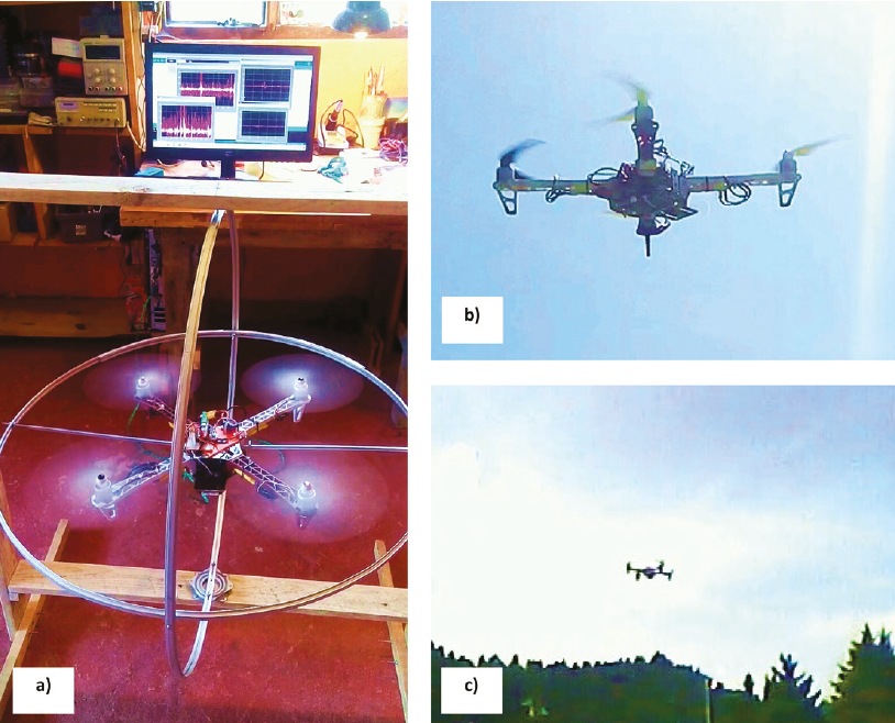
Figure 12:
Experimentation, a) test bench, b) and c) quasi-static flight
Experimentation, a) test bench, b) and c) quasi-static flight
Experimental results on the test bench
The experimental results of the implementation of the controller and filtering stage with the test bench are shown in Figure 13.
Thumbnail

Figure 13:
Results of the experimental stage on the test bench, a) Filtered signal for the pitch angle, b) filtered signal for the roll angle, c) trajectory tracking on the pitch axis, d) trajectory tracking on the roll axis, e) control signal for the pitch movement, f) control signal for the roll movement, g) yaw angle stabilization, h) control signal for the yaw movement
Results of the experimental stage on the test bench, a) Filtered signal for the pitch angle, b) filtered signal for the roll angle, c) trajectory tracking on the pitch axis, d) trajectory tracking on the roll axis, e) control signal for the pitch movement, f) control signal for the roll movement, g) yaw angle stabilization, h) control signal for the yaw movement
Experimental results in quasi-static flight
The experimental results of the implementation of the controller and filtering stage in a quasi-static flight are shown in Figure 14.
Thumbnail

Figure 14:
Experimental results of the quasi-static flight stage. a) Signal filtering for pitch angle, b) signal filtering for roll angle, c) pitch axis stabilization, d) roll axis stabilization, e) control signal for pitch movement, f) control signal for roll movement, g) yaw angle stabilization, h) control signal for the yaw movement
Experimental results of the quasi-static flight stage. a) Signal filtering for pitch angle, b) signal filtering for roll angle, c) pitch axis stabilization, d) roll axis stabilization, e) control signal for pitch movement, f) control signal for roll movement, g) yaw angle stabilization, h) control signal for the yaw movement
Conclusions
In this work, a dynamic model was developed using Euler-Lagrange for a quadcopter type aircraft, then a reduced model was obtained from the complete model, as well as a linear model. Afterward, its open-loop response was compared, observing that for an operating region less than 1 rad, the models behave similarly, later, controllers were designed using the computed torque technique based on the various models and a PID control, the controllers were compared through their performance index, it was determined that anyone controller achieves the objective of stabilizing or tracking the trajectory, later filtering systems were analyzed using observers and Kalman filters, where for each case the three analyzed models were applied, then it was compared the response of the controller and filtering system through a performance index when noise is added to the states and constant disturbances in the parameters, with this it was determined that a linear model is sufficient to design a controller and filtering system, which implies simple implementation and reduction of computational resources for operation with a microcontroller. Additionally, the proposed controller was compared in simulation with a fuzzy logic controller, it was observed that both controllers have similar behavior, however, the proposed controller is easy to implement in a microcontroller, and the stability of the system and filtering is justified with the mathematical analysis presented, against the fuzzy logic controller, for this reason, it was determined to implement the experimental part with said controller. Subsequently, the control and filtering system was implemented for a low-cost IMU and a 32-bit ARM microcontroller, the experimental results showed a behavior similar to the simulation, which validates the use of a linear model to stabilize and track trajectories in the operation of a non-aggressive or aerobatic flight of the aircraft. However, in the experimental part, it was noted that a linear model is sufficient to design the filter and controller, but a control strategy is necessary to give the system robustness to the disturbances caused by the wind or by the disturbances caused by no to know exactly the thrust force of each motor-propeller pair. It is also recommended to design an algorithm that allows improving the performance of the controller estimating the thrust forces of each motor.
References
- Agho, C. (2017). Dynamic model and control of quadrotor in the presence of uncertainties. Links
- Amoozgar, M. H., Chamseddine, A. & Zhang, Y. (2013). Experimental test of a two-stage Kalman filter for actuator fault detection and diagnosis of an unmanned quadrotor helicopter. Journal of Intelligent & Robotic Systems, 70(1-4), 107-117. Links
- Balasubramanian E. & Vasantharaj R. (2013). Dynamic modeling and control of quadrotor. International Journal of Engineering and Technology (IJET), 5(1), 01-07. Links
- Bauer, P. & Bokor, J. (2008). LQ Servo control design with Kalman filter for a quadrotor UAV. Periodica Polytechnica Transportation Engineering, 36(1-2), 9-14. Links
- Beard, R. W. & McLain, T. W. (2012). Small unmanned aircraft: Theory and practice. Princeton university press. Links
- Bouabdallah, S., Noth, A. & Siegwart, R. (2004). PID vs LQ control techniques applied to an indoor micro quadrotor. IEEE/RSJ International Conference on Intelligent Robots and Systems (IROS)(IEEE Cat. No. 04CH37566) 3, 2451-2456. IEEE. Links
- Cárdenas G. (2015). Drones Ciencia al Vuelo. ¿Cómo vez?, UNAM, México, 2015. Links
- Carrillo, L. R. G., López, A. E. D., Lozano, R. & Pégard, C. (2012). Quad rotorcraft control: vision-based hovering and navigation. Springer Science & Business Media. Links
- Castillo, P., García, P., Lozano, R. & Albertos, P. (2007). Modelado y estabilización de un helicóptero con cuatro rotores. Revista Iberoamericana de Automática e Informática Industrial RIAI, 4(1), 41-57. https://doi.org/10.1016/S1697-7912(07)70191-7. Links
- De Jesús-Rubio, J., Cruz, J. H. P., Zamudio, Z. & Salinas, A. J. (2014). Comparison of two quadrotor dynamic models. IEEE Latin America Transactions, 12(4), 531-537. Links
- Elruby, A. Y., El-Khatib, M. M., El-Amary, N. H. & modeling Hashad, A. I. (2012). Dynamic and control of quadrotor vehicle. In The International Conference on Applied Mechanics and Mechanical Engineering 15(5). International Conference on Applied Mechanics and Mechanical Engineering. 1-10. Military Technical College. Links
- Emran, B. J., Al-Omari, M., Abdel-Hafez, M. F. & Jaradat, M. A. (2015). Hybrid low-cost approach for quadrotor attitude estimation. Journal of Computational and Nonlinear Dynamics, 10(3). https://doi.org/10.1115/1.4028524. Links
- Escobedo, J. O., Garcia, E. C., Páramo, L. A., Meda, J. A. & Tapia, R. (2018). Theoretical application of a hybrid observer on altitude tracking of quadrotor losing GPS signal. IEEE Access, 6, 76900-76908. Links
- Euston, M., Coote, P., Mahony, R., Kim, J. & Hamel, T. (2008). A complementary filter for attitude estimation of a fixed-wing UAV. IEEE/RSJ international conference on intelligent robots and systems 340-345. Links
- Falconi, R. & Melchiorri, C. (2012). Dynamic model and control of an over-actuated quadrotor uav. IFAC Proceedings, 45(22), 192-197. Links
- Floreano, D. & Wood, R. J. (2015). Science, technology and the future of small autonomous drones. Nature, 521(7553), 460-466. Links
- Garcia, P. C., Lozano, R. & Dzul, A. E. (2006). Modelling and control of mini-flying machines. Springer Science & Business Media. Links
- Gautam, D. & Ha, C. (2013). Control of a quadrotor using a smart self-tuning fuzzy PID controller. International Journal of Advanced Robotic Systems, 10(11), 380. Links
- Gośliński, J., Giernacki, W. & Gardecki, S. (2013, June). Unscented Kalman Filter for an orientation module of a quadrotor mathematical model. 9th Asian Control Conference (ASCC) 1-6. IEEE. Links
- Gupta, S. G., Ghonge, D. & Jawandhiya, P. M. (2013). Review of unmanned aircraft system (UAS). International Journal of Advanced Research in Computer Engineering & Technology (IJARCET), 2. Links
- Gutiérrez, A. R. H., Duarte, M. A. T. & France, R. G. (2017). El uso de drones en ciencias de la tierra. Links
- Hanley, D. J. & Bretl, T. W. (2016). An improved model-based observer for inertial navigation for quadrotors with low cost imus. In AIAA Guidance, Navigation, and Control Conference 0105. Links
- Hossain R., Rideout D. & Krouglicof N. (2010). Bond graph dynamic modeling and stabilization of a quadrotor helicopter. ResearchGate. Links
- Jung, D. & Tsiotras, P. (2007). Inertial attitude and position reference system development for a small UAV. In AIAA Infotech@ Aerospace 2007 Conference and Exhibit 2763. Links
- Kalman, R. E. (1960). A new approach to linear filtering and prediction problems. Links
- Lendek, Z., Berna, A., Guzmán-Giménez, J., Sala, A. & García, P. (2011). Application of Takagi-Sugeno observers for state estimation in a quadrotor. 50th IEEE Conference on Decision and Control and European Control Conference 7530-7535. IEEE. Links
- Loianno, G., Brunner, C., McGrath, G. & Kumar, V. (2016). Estimation, control, and planning for aggressive flight with a small quadrotor with a single camera and IMU. IEEE Robotics and Automation Letters, 2(2), 404-411. Links
- Macdonald, J., Leishman, R., Beard, R. & McLain, T. (2014). Analysis of an improved IMU-based observer for multirotor helicopters. Journal of Intelligent & Robotic Systems , 74(3-4), 1049-1061. Links
- Markley, F. L. (2003). Attitude error representations for Kalman filtering. Journal of guidance, control, and dynamics, 26(2), 311-317. https://doi.org/10.2514/2.5048. Links
- Muñoz, L. E., Castillo, P. & García, P. (2013). Observer-control scheme for autonomous navigation: Flight tests validation in a quadrotor vehicle. International Conference on Unmanned Aircraft Systems (ICUAS) 95-804. IEEE. Links
- Nonami, K., Kendoul, F., Suzuki, S., Wang, W. & Nakazawa, D. (2010). Introduction. In Autonomous Flying Robots. Japan: Springer. 1-29. Links
- Noordin, A., Basri, M. A. M. & Mohamed, Z. (2018). Sensor fusion algorithm by complementary filter for attitude estimation of quadrotor with low-cost IMU. Telkomnika, 16(2), 868-875. Links
- Paiva-Peredo, E. A. (2016). Modelado y control de un cuadricóptero. Links
- Patete, A. & Erazo, A. (2016). Linear and nonlinear control for a micro unmanned aerial vehicle with quadrotor configuration. Revista Ingenierıa UC, 23(3), 247-259. Links
- Raffo, G. V. (2007). Modelado y Control de un Helicóptero Quad-Rotor. MS, disertación, Dept. telemática, automática y robótica, Univ. de Sevilla. https://www.researchgate.net/deref/http%3A%2F%2Fdx.doi.org%2F10.1109%2FIROS.2007.4399042. Links
- Reyes, F. (2011). Robótica-control de robots manipuladores. Alfaomega grupo editor. Links
- Roldan-Caballero A. (2016). Modelado y monitoreo para un drone tipo cuadrirotor (Tesis de Maestría en Ingeniería de Manufactura). Instituto Politécnico Nacional. Ciudad de México. Links
- Rodríguez R., Ipanaqué W., Carrera E. (2016).Comparación de modelos matemáticos y controladores PID vs LQR para un cuadricóptero. Universidad de Piura, Facultad de Ingeniería. Links
- Sabatino, F. (2015). Quadrotor control: modeling, nonlinearcontrol design, and simulation. Links
- Sadr, S., Moosavian, S. A. A. & Zarafshan, P. (2014). Dynamics modeling and control of a quadrotor with swing load. Journal of Robotics, 2014. https://doi.org/10.1155/2014/265897. Links
- Sanz, R., Ródenas, L., García, P. & Castillo, P. (2014). Improving attitude estimation using inertial sensors for quadrotor control systems. International Conference on Unmanned Aircraft Systems (ICUAS) 895-901. IEEE. Links
- Sarim, M., Nemati, A., Kumar, M. & Cohen, K. (2015). Extended kalman filter based quadrotor state estimation based on asynchronous multisensor data. In Dynamic Systems and Control Conference 57243. American Society of Mechanical Engineers. https://doi.org/10.1115/DSCC2015-9929. Links
- Sebesta, K. D. & Boizot, N. (2013). A real-time adaptive high-gain EKF, applied to a quadcopter inertial navigation system. IEEE Transactions on Industrial Electronics, 61(1), 495-503. Links
- Sevilla, L. (2014). Modelado y control de un cuadricóptero. Universidad Pontificia de Comillas. Links
- Shi, D., Wu, Z. & Chou, W. (2018). Generalized extended state observer based high precision attitude control of quadrotor vehicles subject to wind disturbance. IEEE Access , 6, 32349-32359. Links
- Simon, D. (2006). Using nonlinear Kalman filtering to estimate signals. Embedded Systems Design, 19(7), 38. Links
- Sira-Ramírez, H. E. B. E. R. T. T., Márquez, R., Rivas-Echeverria, F. & Llanes-Santiago, O. (2005). Control de Sistemas no lineales. Automática & Robótica. Pearson Educación SA. Links
- Tailanián, M., Paternain, S., Rosa, R. & Canetti, R. (2014). Design and implementation of sensor data fusion for an autonomous quadrotor. IEEE International Instrumentation and Measurement Technology Conference (I2MTC) Proceedings 1431-1436. IEEE. Links
- Xiong, J. J. & Zheng, E. H. (2015). Optimal kalman filter for state estimation of a quadrotor UAV. Optik, 126(21), 2862-2868. Links
- You, W., Li, F., Liao, L. & Huang, M. (2020). Data Fusion of UWB and IMU Based on Unscented Kalman Filter for Indoor Localization of Quadrotor UAV. IEEE Access , 8, 64971-64981. Links
- Yu, J., Shi, P., Dong, W. & Yu, H. (2015). Observer and command-filter-based adaptive fuzzy output feedback control of uncertain nonlinear systems. IEEE Transactions on Industrial Electronics , 62(9), 5962-5970. Links
- Yoo, T. S., Hong, S. K., Yoon, H. M. & Park, S. (2011). Gain-scheduled complementary filter design for a MEMS based attitude and heading reference system. Sensors, 11(4), 3816-3830. Links
Annexed
Glossary
Q: is the covariance of the noise process
R: is the covariance of the noise in the measurement
I: is the identity matrix.