


 nueva página del texto (beta)
 Inglés (pdf)
 Artículo en XML
 Referencias del artículo
 Enviar artículo por email
 Citado por SciELO
  Similares en
SciELO
Similares en
SciELO 
 Permalink
1 Introduction
Sorption is of great value for the purification of waters and industrial effluents containing contaminants or pollutants. The modeling of the kinetics is important for the prediction of uptake rates and for gaining more insight into the mechanisms. However, this is still a discussed problem (Qiu et al., 2009). Moreover, a particular situation prevails in this field, which may be viewed as follows.
It has long been recognized that most sorption processes in macroscopic adsorbent beads are controlled by diffusion in the particles, or in a layer at the periphery of the particles (Ruthven, 1984; Do, 1998). Apparently (Do, 1998), this hypothesis was put forward for the first time nearly one century ago by McBain on the basis of experiments with carbon (McBain, 1919). It was also first recognized by Boyd (Boyd et al., 1947) in the case of ion exchange (Liberti and Helfferich, 1983). In an article published in 1965, Helfferich started by stating: "It has long been known that ion-exchange rates are controlled by diffusion" (Helfferich, 1965).
Consequently it is surprising that descriptions of experimental results based on a rate-limiting equation for the adsorption reaction have become increasingly popular in the past 30 years (Ho and McKay, 1999). These empirical equations include the pseudo-firstorder (Lagergren, 1898) and the pseudo-second-order rate law (Blanchard et al., 1984; Gosset et al., 1986). Other more physical descriptions assumed a mixed regime combining diffusion and local adsorption reaction (Wen, 1968; Yang and Al-Duri, 2001; Che Galicia et al., 2014; Castillo-Araiza, 2015).
The other formula that is usually tested against the chemical rate laws is the "intra-particle diffusion" (IPD) equation (Kushwaha et al., 2010; Boparai et al., 2011; Tofighy and Mohammadi, 2011) which is supposed to be relevant in the case of diffusioncontrolled sorption processes (Weber and Morris, 1963; Rudzinski and Plazinski, 2008; Wu et al., 2009; Haerifar and Azizian, 2013). This equation was first employed by Boyd et al. in 1947 (Boyd et al., 1947) to model ion exchange kinetics in zeolites. However, this formula was established originally to describe pure free diffusion of a solute in a sphere (see for instance Eq. (6.20) of (Crank, 1975)). It does not account explicitly for the effect of adsorption.
In the present work we focus on diffusioncontrolled adsorption processes and propose to revive a model that takes into account the influence of adsorption on solute transport in the adsorbent. This model was first proposed in the seminal work by Crank (Crank, 1957, 1975). When applied to sorbent spherical beads, it is an example of the well-known so-called "shrinking unreacted core" model (Yagi and Kunii, 1961; Ruthven, 1984; Levenspiel, 1999; Leyva-Ramos et al., 2010, 2012, 2015) in which adsorption of the diffusing solute progressively builds up an ash shell of reacted material at the periphery of the bead and leaves an unreacted core at the centre, that shrinks in the course of time. The model introduced by Crank was solved in the case of a very large (virtually infinite) amount of solute, in which the external solution concentration could be taken as constant (Crank, 1957, 1975; Ruthven, 1984; Levenspiel, 1999). In practice, this model should be applicable when the solute concentration in the batch adsorber is sufficiently large (see section 2).
In this paper, we first recall briefly the main ingredients and results of the model in one dimension (1D). The method used here serves to gain more insight into the main features of the process. Next, the model is solved in the case of spherical beads for a finite amount of adsorbate present initially in the batch adsorber, in which case its bulk concentration varies with time. The result is used to derive a formula valid at short contact times, for particles of arbitrary (but smooth) shape, and for a discussion of the IPD equation. It is shown that the diffusion coefficient introduced in the IPD equation is in fact a lumped parameter that, besides diffusion, also includes the effect of the experimental conditions. The conditions required for applying the model to real experiments are discussed. The obtained formulas are utilized to describe experimental data taken from the literature.
2 Modeling
2.1 Ingredients of the model
We consider an adsorbent medium (denoted by A) in contact with a perfectly stirred batch adsorber, denoted by B, containing all of the solute initially. The adsorbate diffuses freely in A until it is immobilized when it encounters a free site.
As shown in the literature (Ruthven, 1984; Grathwohl, 2012), in the case of very low concentration of solute, the latter obeys a diffusion equation with an effective diffusivity, De f f = D(1 + α) (Ruthven, 1984; Grathwohl, 2012), in which D is the diffusivity of free solute and ? is the slope of the adsorption isotherm for very low concentration.
On the opposite, in the present work, the initial concentration in the batch adsorber will be sufficiently high so that the ash layer of the adsorbent operates in the plateau region of the adsorption isotherm. In this case, the degree of adsorption in the reacted zone will not vary appreciably in the course of time as long as the external concentration remains high enough.
In the model, the medium will be considered to possess a uniform concentration of sites, denoted by Cs , onto which the solute molecules form a monolayer. It will be supposed that the adsorption process is diffusion-controlled, i.e. the adsorption process is very fast compared to diffusion. The latter will be described by using an average diffusion coefficient in A, which will account for the various possible diffusion pathways in the medium (micropore, mesopore, macropore, and surface diffusion (Do, 1998)). The total amount of solute will be sufficiently high so that the ash layer thickness in A at equilibrium is not very small. So, the concentration of solute on the surface of A will be taken equal to that in the batch adsorber, denoted by CB . The boundary condition for the solute concentration in A will be that the concentration of free solute is continuous at the mouth of a pore.
The classic quasi-steady state (QSS) approximation (Briggs and Haldane, 1925; Kramers, 1940; Crank, 1975; Simonin et al., 1991) will be used to derive analytical results. Generally, the QSS regime does not hold at the very beginning of the process, but it settles after a short induction time.
2.2 Adsorption in a semi-infinite slab (1D case)
Before examining the spherical case, it is useful to first present shortly the model introduced by Crank (Crank, 1957, 1975) in the one-dimensional (1D) case and solve it in the QSS approximation because this has not been done before in the literature and some results will then be used for the spherical case. Moreover this derivation gives more insight into the process.
We consider a semi-infinite porous slab of adsorbent that is put in contact at t = 0 with a very large bath of batch adsorber of constant concentration,

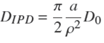
The concentration of free solute, C(x,t), in this zone obeys Fick's second law which reads ∂C(x,t)/∂t = −∂J(x,t)/∂x = D∂2 C(x,t)/∂x 2, with t the time, D the diffusion coefficient of the adsorbate in A, and J the flux of solute molecules per unit cross-section area given by Fick's first law, J(x,t) = −D∂C(x,t)/∂x. It results from the definition of δ1 that C = 0 at x = δ1.
The variation of δ1 in a time interval dt is given by the relation,
 (1)
(1)
which expresses the fact that the variation of the number of occupied sites in the lapse of time dt is equal to the number of solute molecules arriving at the position x = δ1 at time t. At this location, the adsorbent acts like a sink for the solute.
In the QSS approximation one has,
∂C(x,t)/∂t
≈ 0 in the ash layer (and C = 0 for x >
δ1). Then
J(x,t) is approximately
constant in space in this layer by virtue of Fick's second law, so that
J = J(t). Consequently,
the concentration profile is approximately linear in this zone because of Fick's
first law. Because of the boundary condition, C =
p
 (2)
(2)
By combining Eqs. (1) and (2) one gets the equation,
 (3)
(3)
which yields,
 (4)
(4)
with
 (5)
(5)
and
 (6)
(6)
the effective diffusion coefficient in the porous adsorbent. In what follows it will be taken as a constant because the solute concentration will be very low (see Results and discussion section). The total uptake of solute by A (per unit cross-section area) is
 (7)
(7)
because in practical applications one may neglect the concentration of free solute in A as compared to that of adsorbed solute. Therefore one gets from Eqs. (4)-(7),
 (8)
(8)
We notice that in this relation Q varies as
2.3 Adsorption in spherical beads
We now consider sorbent spheres of radius R that are immersed at t = 0 in a well-stirred batch adsorber of initial concentration
In this section, we use the same type of model as in the 1D case. Its application to adsorption in spheres has been solved in the literature in the case of an infinitely large amount of solution, in which the adsorbate concentration remained constant (Crank, 1957, 1975; Levenspiel, 1999). It is solved below in the case of a finite amount of adsorbate, whose bulk concentration varies with time.
Let us define the maximum site occupancy ratio of a sphere as the ratio of the total number of solute molecules to the total number of sites,
 (9)
(9)
with v the volume of a sphere and VB the volume of batch adsorber per sphere (volume of the bath divided by the number of spheres).
A spherical bead is depicted in Fig. 2. We denote by r 0 the position of the moving boundary delimiting the shrinking unreacted core, at which the concentration of free solute concentration vanishes, and by δ the thickness of the ash (reacted) shell.

The free solute concentration at position r and time t,C(r,t),obeys Fick's law, ∂u/∂t=D∂2 u/∂r 2,with u≡ rC(r,t) (Crank, 1975). The QSS approximation in the sphere reads: ∂u/∂t ≈ 0. Then, using the latter relation and the boundary condition, C(r = R−,t) = pCB , and solving Fick's law one obtains,
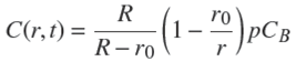 (10)
(10)
The relation for the time variation of r0, similar to EQ.(1), reads,
 (11)
(11)
in which n is the number of moles of solute arriving at r0 and the flux per unit cross-section area is given by J = −D∂C/∂r.
It stems from Eqs. (10) and (11) after a simple manipulation that,
 (12)
(12)
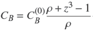
in which CB
is obtained from the conservation of total solute amount in the course of time:
 (13)
(13)
in which we also used Eq. (7). Then one gets,
 (14)
(14)
in which we have used Eq. (9) and introduced the non-dimensional radius of the core,
 (15)
(15)
Insertion of Eq. (14) into Eq. (12) gives the following separable differential equation obeyed by ɀ,
 (16)
(16)
with a defined by Eq. (5). The two sides of this equation can be integrated separately (e.g. with the help of Maple), between the states (t = 0, ɀ = 1) and (t,ɀ(t)). After some rearrangements of terms, one arrives at the following result,
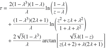 (17)
(17)
in which
 (18)
(18)
is a non-dimensional reduced time, and the parameter λ defined by,
 (19)
(19)
has been introduced for convenience. In practice, one generally has ρ < 1. Then it is easy to show that the minimum value of ɀ satisfies the relation, ρ = 1 − ɀ 3 min, from which one gets using Eq. (19),
 (20)
(20)
which expresses the concrete meaning of the parameter ג.
The fractional uptake (proportion of solute immobilized in the sphere) is (Do, 1998),
 (21)
(21)
By using Eqs. (9), (13) and (15) in Eq. (21) one gets,
 (22)
(22)
from which it stems that,
 (23)
(23)
Therefore, τ can be expressed as a function of P and ρ alone by inserting Eqs. (19) and (23) into Eq. (17).
2.4 Formula at short times
For small diffusion times, P is small. In that case, one gets from Eq. (23) that ɀ ≈ 1 − ρP/3, which relation may be inserted into Eq. (17). A Taylor expansion of this expression for τ to the second order in powers of P leads to
 (24)
(24)
or, together with Eqs. (5) and (9),
 (25)
(25)
In fact, Eq. (25) may be obtained in another way, by noting that for small contact times the solute is adsorbed in a shell of small thickness given by the formula in 1D (Eq. (4)) and area 4πR 2, so that, Q ≈ Cs 4πR 2 δ1 , which together with Eq. (21) leads to Eq. (24) or (25).
Moreover, as a consequence, we notice that this treatment may be applied to particles of arbitrary, yet smooth, shape in the first moments of the process. Then, the amount of solute adsorbed in the particle is given by,
 (26)
(26)
with A the area of the particle, and consequently,
 (27)
(27)
An important result of this latter formula is that the fractional uptake, P, not only varies as t
1/2. It is also noticed that P should decrease with
2.5 Intraparticle diffusion equation
The classic intraparticle diffusion (IPD) equation (Boyd et al., 1947; Weber and Morris, 1963; Rudzinski and Plazinski, 2007; Wu et al., 2009) in the case of a sphere is expressed as,
 (28)
(28)
in which PIPD
is the fractional uptake of solute, QIPD
is the uptake,
It seems that this relation was first used by Boyd et al. (1947) to describe adsorption kinetics in zeolites. However, as said previously, it does not take into account explicitly the effect of adsorption. It is the solution to the problem of free diffusion of a solute from a batch adsorber of constant concentration into a sphere that does not possess adsorption sites (Eq. (6.20) of (Crank, 1975)).
At the beginning of the process, Eq. (28) may be approximated by the following equation (Crank, 1975; Rudzinski and Plazinski, 2007),
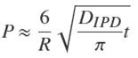 (29)
(29)
In the literature, the IPD equation has generally been used in the latter form preferentially to the full formula, Eq. (28). It is worth noting that Eq. (29) coincides with the result from the present model, Eq. (24), that is PIPD ≈ P at short times, provided that the diffusion coefficient appearing in the IPD equation satisfies the relation,
 (30)
(30)
or, by using Eqs. (25) and (29),
 (31)
(31)
This result shows that the IPD diffusion coefficient is in fact a lumped parameter which depends on the experimental conditions. In particular, within the present model, for a given type of sorbent particles and a given volume of bath per particle, this pseudo-diffusion coefficient is expected to be inversely proportional to
WhenDIPD is given by Eq.(30), then P ≈Pat short times, but PIPD becomes larger than P for longer times. It was observed that the maximum deviation grows with the value of ρ. It reaches 7.2% for ρ = 0.1, ca.13% for ρ=0.5 and ca. 20%forρ=0.9.
2.6 Application of the model to experiments
The value for the concentration of sites, Cs, to be taken in the model must be determined. To illustrate, let us assume that the adsorption isotherm of A may be parameterized using the Langmuir equation, which is generally written as,
 (32)
(32)
with qa the amount of solute adsorbed in A per mass unit of A,
This relation may be rewritten in the following different form,
 (33)
(33)
with qsat
= KL
/aL
the amount at saturation and C
1/2 = 1/aL
. This form expresses the fact that
If the adsorption process is sufficiently fast, one may assume a local equilibrium in a pore between the free solute and the solute adsorbed on the wall of the pore. Then, Eq. (33) may be extended to express the space-averaged concentration of adsorbed solute at a position in a pore as,
 (34)
(34)
in which Csat
is the space-averaged concentration of adsorbed solute in A at saturation and C′ is the real free solute concentration in the pore, C′ = C/p. If qsat is the mass of solute adsorbed per mass unit of adsorbent, then Csat
= qsatd, with d the apparent density of the adsorbent particles. In passing from Eq. (33) to Eq. (34), it is assumed that the concentration of free solute in the pores is equal to that in the external bath
If the initial concentration of solute in the batch adsorber,
In the present study, a natural choice for the effective value of CS was the value of the adsorbed concentration of solute at equilibrium for a representative value of the solute concentration in the pores, C0, that is,
 (35)
(35)
In wich Cα is given by Eq. (34). A sensible choice for
3. Results and discussion
3.1 Description of experimental results
First, the accuracy of the analytical expressions derived assuming a QSS in the adsorbent was examined through comparison with results from finitedifference (FD) calculations in the case of constant external concentration. The FD algorithm was based on a diffusion-equilibration scheme used in previous work (Simonin et al., 1988). The main result is that the QSS hypothesis is valid, and the analytical expressions are accurate, when a ≤ 0.1.
Then, the results obtained in this work were applied to describe experimental results. The variation of the kinetics with the initial bulk adsorbate concentration and the validity of the predictions found in the theoretical section were examined. Kinetic data were found for various adsorbents, including chitosan (Wu et al., 2001), resin (Hosseini-Bandegharaei et al., 2010), fly ash (Panday et al., 1985), home made activated carbon (Demirbas et al., 2008; Periasamy and Namasivayam, 1996; Santhy and Selvapathy, 2006) and commercial activated carbon (Kumar et al., 2003; Choy et al., 2004; Yang and Al-Duri, 2001, 2005).
The present model is not supposed to be applicable to systems in which ion exchange is the mechanism of adsorption because this process involves electric coupling between the diffusing ions. This is what we found when we analyzed for instance the data about the adsorption of Pb(II) in an algae gel (Vilar et al., 2007). It was observed that P varied approximately as t but it did not vary as
On the other hand, satisfactory results were found in the case of experiments carried out with commercial carbon like Filtrasorb. Hereafter, we present an analysis of the data reported by Choy et al. (Choy et al., 2004), and by Yang and Al-Duri (Yang and Al-Duri, 2001) about the adsorption of two different dyes, acid yellow 117 and Cibacron reactive yellow F-3R (RY, molar mass ~ 712 g mol−1), respectively, in porous beads of activated carbon, Filtrasorb 400 (F400). The data of Yang and AlDuri were particularly interesting because the main physical-chemical characteristics of the beads have been reported. Besides these results with Filtrasorb carbon, we present in the next section the result obtained in the case of the adsorption of Cu(II) on chitosan (Wu et al., 2001) at short times.
The numerical values for the experimental kinetic measurements were obtained by digitizing the figures presented in the references.
3.1.1 Analysis of data at short times: variation of P with time and
Experimental data may be represented using the approximate expression, Eq. (24) or (27), at short times, when the adsorption rate P is typically smaller than ~0.3 or 0.4 (Rudzinski and Plazinski, 2007, 2008).
It was first interesting to study the effect of varying the initial external concentration in (Choy et al., 2004) and (Yang and Al-Duri, 2001). In these two references the initial bulk concentrations of the adsorbate were appreciably larger than C
1/2. One gets from Table 3 of (Choy et al., 2004) that C
1/2 ≈ 4.6 ppm, which is indeed much smaller than all initial concentrations
In the experiments of (Choy et al., 2004), most of the values of the fractional uptake did not exceed 0.4, so that the approximate expression for P (Eq. (27)) was sufficient to analyze nearly all of the data. In (Yang and Al-Duri, 2001), the fractional uptake nearly reached its equilibrium value at the end of the experiments. Next, these data were analyzed here at short times and, besides, in the whole time range.
The results for the analysis of the fractional uptake P as a function of the square root of time are shown in Fig. 3 and Fig. 4.

Fig. 3 Sorption rates as a function of time in rates as a function of time in the experiments of (Choy et al., 2004) for various initial concentrations of solute in the bath. Upper plot: experimental values of P vs. t
1/2; bottom plot: experimental values of

Fig. 4 Sorption rates as a function of time in the experiments of (Yang and Al-Duri, 2001) for various the experiments of (Choy et al., 2004) for various initial concentrations of solute in the bath. Upper plot: experimental values of
The upper frames show the variation of P as a function of
The bottom frames show the plots of the function
Besides these findings in the case of a commercial activated carbon (Filtrasorb), experimental data were analyzed in the case of other materials, spanning a wide range of viable sorbent types, namely for dyes and Cu(II) in home-made activated carbons (Demirbas et al., 2008; Santhy and Selvapathy, 2006; Periasamy and Namasivayam, 1996); and for Cu (II) in a resin impregnated with an extracting (Hosseini-Bandegharaei et al, 2001), and in fly ash (Panday et al, 1985). Inmost cases, the fractional uptake was found to vary as
However, the case of the data for Cu(II) in chitosan (Wu et al., 2001) gave an interesting result, which is shown in Fig. 5. The mechanism proposed in this reference (Wu et al., 2001) for the adsorption of Cu(II) was the chelation by unprotonated amino groups of chitosan, without ion exchange.

Fig. 5 Sorption rates as a function of time in the experiments of (Wu et al., 2001) for various initial concentrations of solute in the bath. Upper plot: experimental values of P vs. t
1/2; bottom plot: values of
It is seen in this figure that the experimental points for
3.1.2 Analysis of data in the whole time range
The experimental results of (Yang and Al-Duri, 2001) were also described in the whole time range by using the full equation, Eq. (17), together with Eqs. (19) and (23). For this purpose, the values of α and ρ were determined as follows. One gets the value of qsat in Eq. (33): qsat
= KL/aL ≈ 199 mg g−1, from which one obtains the value of Csat in Eq. (34): Csat = 199 g L−1 (with d = 1 g mL−1 (Chang et al., 2004)). For each initial concentration
Table 1 Values of input parameters in the model (in Eq. 17) for the data of (Yang and Al-Duri, 2001) for RY of molar mass ~ 712 g mol-1, and for which R=0.0536 cm and Csat= 279.6 mol m-3.

Eq. (17), together with Eqs. (19) and (23), was used to calculate the concentration of solute remaining in the batch adsorber, CB , as a function of time for various initial bulk concentrations. The value of D0 was optimized 'manually' by plotting the experimental points together with the results from the model. The plots for CB are shown in Fig. 6 for a common value, D 0 = 5.83×10⁻¹² m2 s−1 or D = 1.08×10⁻¹¹ m2 s−1 because of Eq. (6) with the value for the porosity, p1/=2 0.54 (Chang et al., 2004). We are not aware of any direct true diffusion coefficient measurements in porous carbon. However, some diffusivity values have been reported recently, that were obtained from the use of true diffusional models (not from the IPD equation): D of the order of 3 × 10⁻¹⁰ m2 s−1 for the fluoride ion in bone char (Leyva-Ramos et al., 2010); of a few 10−11 m2 s−1 for pyridine in activated carbon (Leyva-Ramos et al., 2015) and for Rhodamine B in a zeolite (Castillo-Araiza et al., 2015); and D in the range from 0.5 × 10⁻¹² m2 s−1 to 27 × 10−12 m2 s−1 for various organic compounds in activated carbon (Leyva-Ramos et al., 2012). Our value D = 1.08 × 10⁻¹¹ m2 s−1 therefore falls in the range of values obtained in these references. Besides, the diffusivity value of RY in bulk water should be of the order of a few 10−10 m2 s−1, as found by using the Stokes-Einstein formula (D = kBT /6πηR) at 25°C with a radius of the order of 8-10 Å for the solute molecule. Then, it is plausible that this value may be reduced by a factor of several tens because of effects due to tortuosity, and to confinement in the micropores which constitute the major part of the pores in F400 carbon (Chang et al., 2004).

Figure 6 Concentration of solute remaining in the batch adsorber as a function of time in the experiment of (Yang and Al-Duri, 2001) for several values of the initial concentration and a diameter of 0.0536 cm. Symbols: (∙)
It is seen in Fig. 6 that the model gives results in rather good agreement with experiments for the 4 initial concentrations, with
The agreement with experiment is a little less accurate than that reported in (Yang and Al-Duri, 2001) in the framework of the branched pore diffusion model. However, this latter treatment involved 4 adjustable parameters instead of only one here (D).
Conclusion
In this work we have used an intraparticle diffusionadsorption model to describe diffusion-controlled adsorption kinetics. It is expressed in terms of measurable physicochemical parameters. In principle, it is free of any adjustable parameter. However, the solute diffusion coefficient in the adsorbent must be available, which is generally not the case. Moreover, it is difficult to measure experimentally. Then D is the only unknown parameter.
An approximate solution was obtained for short diffusion times, which has the same form as the classical IPD equation, i.e. it varies as t 1/2. It has been shown that the diffusion coefficient introduced in the IPD equation is a lumped parameter. According to the present model, this pseudo-diffusion coefficient should decrease with the initial solute concentration in the bath, as the inverse square root of this concentration. Such a decrease has been observed experimentally in the literature.
The best adsorbents for the application of the present model are those in which the mechanism of sorption is not ion exchange. The model may be used when the external solute concentration is in the plateau region of the adsorption isotherm of the material.
At a more general leve, it may be put forward that rate control by a chemical reaction is unlikely, especially in the (most frequent) case of sorbent particles of macroscopic size, in which complete adsorption takes an appreciable time (hours or sometimes days). On the other hand, limitation by a chemical reaction, or mixed chemical-diffusion control, may occur in the case of particles of small size in which diffusive transport may be fast (as e.g. in (Sharma et al., 1990)). It should also be recollected that the best way to discriminate between chemical and diffusion control is to carry out experiments with beads of various sizes. Indeed, as underlined long ago by (Boyd et al., 1947), the size of the adsorbent particles should have no influence on the uptake rate if adsorption is controlled by a chemical reaction, so long as the mass of adsorbent is kept constant. Furthermore, the shape of the particles should have no influence in this case, which is a very useful feature.
Nomenclature
a |
|
a L |
Langmuir isotherm parameter, m3 kg−1 |
A |
area, m2 |
C |
concentration of free solute, mol m−3 |
C a |
concentration of adsorbed solute, mol m−3 |
|
mass concentration of solute in batch adsorber at equilibrium, kg m-3 |
|
concentration of solute in batch adsorber, mol m−3 |
C S |
concentration of adsorption sites, mol m−3 |
C 1/2 |
mass concentration of solute in batch adsorber at which qa = qsat/2, kg m−3 |
C ' |
mass concentration of free solute in pore, kg m−3 |
C ' 0 |
mean mass concentration of free solute in pore, kg m−3 |
D |
diffusivity of solute in sorbent, m2 s−1 |
D IPD |
IPD diffusivity of solute in sorbent, m2 s−1 |
D 0 |
effective diffusivity of solute in sorbent (Eq. (6)), m2 s−1 |
J |
flux of solute per unit area, mol s−1 m−2 |
K L |
Langmuir isotherm parameter, m3 kg−1 |
n |
solute mole number, mol |
p |
porosity, adimensional |
P |
fractional uptake, adimensional |
q a |
mass of solute adsorbed per mass of A, adimensional |
q sat |
mass of solute adsorbed per mass of A at saturation, dimensionless |
Q |
quantity of adsorbed solute, mol |
|
quantity of solute in batch adsorber at t = 0, mol |
Q IPD |
quantity of adsorbed solute in IPD equation, mol |
r |
radial coordinate in sphere, m |
r 0 |
radius of shrinking core, m |
R |
sphere radius, m |
t |
time, s |
v |
volume of sphere, m3 |
V B |
volume of solution, m3 |
x |
space coordinate, m |
ɀ |
reduced radius ≡ r0 /R, dimensionless |

