1. Introduction
This work intends to jointly decide the frequency of delivery and rotation cycle time for a multiproduct producer-retailer integrated system featuring overtime and scrap. To meet the increasing demands on diversity of end items, production managers today constantly require a multiproduct fabrication plan. Dixon and Silver (1981) examined an optimal lot-size problem with one work center that produce multiproduct. The known period by period demands for each item were assumed for a finite period of time. Setup costs were fixed and the fabrication and holding costs were assumed to be linear. These costs were varied for different products. Their goal is to decide batch size so that (i) total costs can be kept minimum; (ii) no shortage occurs; and (iii) capacity does not exceed. A heuristic was proposed to decide the feasible solution, and examples were used to show that their heuristic in most circumstances can provide good solution with a relatively short computer time. Mitchell (1988) proposed an algorithm based on the generalized Knapsack duality algorithm to study a multi-item inventory system with service level constraint. The objective was to locate the system’s approximate optimal policies. As a result, it pointed out that by applying the proposed model, the operating expense can be considerably cut down as compared to the existing uniform service model. Sambasivan and Schmidt (2002) solved the multi-plant, multiproduct, capacitated lot-size problems with inter-plant transfers. To tackle the problems, they proposed a heuristic procedure starting with solution to un-capacitated problem. They further used a smoothing routine to eliminate any violations of capacity. Broad experimentations were performed to verify accurate of their heuristic results, which were executed on IBM mainframe environments. Sancak and Salmann (2011) determined the optimal purchasing and inbound receiving policies for a producer that acquires multi-item from a provider. Their objective was to meet the needs in fabrication plan over a finite period of times, and to lower the total delivery and stock holding expenses. The delivery cost per truck is charged to the producer. They proposed an idea of shipping a full truckload as needed and used safety stocks to cover those requirements that are less than a full truckload. The influences of such a delay shipping on the service levels and related cost were analyzed. It pointed out that the proposed idea considerably cut down the delivery and stock holding costs. Chiu et al. (2016) investigated a two-machine multiproduct finite production rate model considering delayed differentiation, scrap, and multi-shipment policy. A cluster of multiproduct that shares a component and two-phase fabrication procedures are assumed. In phase 1 only the mutual components are produced by machine 1; while in phase 2, a separate machine fabricates the diverse end products. The objectives were to simultaneously reduce manufacturing time and overall system costs. Their results were compared to both single-phase and two-phase single-machine schemes, to demonstrate the merits of their proposed scheme. Extra articles that explored diverse aspects of multiproduct replenishment systems and/or supply chains can be found elsewhere (Barata, 2021; Benítez, 2019; Chiu et al., 2020; Chiu, S. et al., 2021; Farmand et al., 202; Kumar et al., 2019; Lin et al., 2019; López-Ruíz, & Carmona-Pourmohammadi et al., 2020; Raza & Govindaluri, 2019).
Random defects often exist in real fabrication processes due to different uncontrollable causes. Eroglu and Ozdemir (2007) studied an economic order quantity (EOQ) model featuring defects and backlogging. All items are screened to identify defects and scraps from perfect goods. Impact of defect rate on EOQ was investigated. Moussawi-Haidar et al. (2013) examined an EOQ system with unreliable supplier. Acceptance sampling policy was used toward every incoming order to determine whether a follow-up 100% inspection is required or not (it is required only if outcomes of quantity of imperfect goods in sampling plan exceeds the acceptable standard). Non-linear math program is formulated that combines the stock refilling and quality issues into a profit model in order to simultaneously decide the best lot size and sampling plan, which help achieve the desirable average outgoing quality limit. A procedure along with numerical illustration was provided to jointly calculate the optimal lot size and sampling plan to the problem and demonstrate applicability and performance of their results. Additional studies (Afshar-Nadjafi et al., 2019; Bhagat et al., 2021; Chiu, Lin, & Wu, 2020; Daryanto, & Christata, 2021; Hariga & Ben-Daya, 1998; Lesmono et al., 2020; Mokao, 2020; Sana, 2010; Terdpaopong et al., 2021; Yamada et al., 2021) also focused on different features of imperfection products and/or manufacturing systems.
Further, an overtime option is usually treated as an effective means to expedite fabrication processes/time, so as the demands can be met sooner. Makino and Tominaga (1995) indicated that the estimation of periodic fabrication quantity (e.g. by month or by year) is required initially to plan production of a new product. Secondly, to design and construct a standardized flexible assembly system which includes numerous sub-systems (such as feeding, moving work-in- process, assembly, etc.) is necessary for meeting the required cycle time. Accordingly, they estimated and discussed both fabrication rate and the required cycle length for a classic flexible assembly system. El-Gohary et al. (2009) applied the optimal control theory to adjust the fabrication rate for a deteriorating inventory system, wherein a manufacturing firm makes certain items at a constant rate and is intended to improve its fabrication rate. An optimal control model was constructed/formulated to deal with the problem, and as a result, an explicit solution along with illustrative example was presented to show applicability of the obtained results. Extra papers (Campbell, 2017; Chiu et al., 2020; Chiu, Y. et al., 202; Chiu, Lin, & Wu, 2020; Ivanov et al., 2019; Lin et al., 2019; Lesmono et al., 2020; Mokao, 2020; Nicolaisen, 2011; Ohmori & Yoshimoto, 2021;) also addressed systems with overtime options and adjusted fabrication/output rates. This study intends to jointly decide the rotation cycle length and frequency of delivery for a multiproduct producer-retailer integrated system featuring overtime and random scrap.
2. The multiproduct producer-retailer integrated system
2.1. List of notation
L= |
total number of different products to be produced in the proposed study, |
λi = |
annual demand of product i (where i equals to 1, 2, …, L), |
Qi = |
lot size of product i, |
TA= |
rotation cycle time - decision variable, |
n= |
number of deliveries per cycle - a decision variable, |
P1iA = |
annual manufacturing rate of product i when overtime is implemented, |
P1i = |
standard annual manufacturing rate of product i without overtime option, |
α1i= |
added proportion of production rate due to overtime implementation (where α1i > 0), |
CiA = |
unit production cost of product i when overtime is implemented, |
Ci = |
standard unit cost of product i without overtime option, |
α3i= |
connecting factor between Ci and CiA (where α3i > 0), |
KiA = |
setup cost of product i when overtime is implemented, |
Ki = |
standard setup cost of product i without overtime option, |
α2i = |
connecting factor between costs of Ki and KiA (where α2i > 0), |
t1iA = |
production uptime of product i, |
t2iA = |
delivery time of product i, |
hi = |
unit holding cost of product i, |
h2i = |
unit holding cost of product i at the retailer’s side, |
xi = |
random scrap rate of product i fabricated in production process, |
E[xi ] = |
the expected scrap rate of product i, |
d1iA = |
manufacturing rate of scrap product i during uptime, |
CSi = |
unit disposal cost of product i, |
Hi = |
stock level of perfect product i at the end of its uptime, |
K1i = |
fixed shipping cost of product i, |
CTi = |
unit delivery cost of product i, |
tniA = |
fixed time interval between two successive deliveries of product i, |
T= |
rotation cycle time in the same system without overtime, |
t1i = |
uptime of product i in the same system without overtime, |
t2i = |
delivery time of product i in the same system without overtime, |
d1i = |
production rate of scrapped product i in the same system without overtime option, |
I(t)i = |
level of end product i at time t, |
ID(t)i = |
level of scrapped product i, |
IC(t)i = |
stock level of product i at retailer side, |
E[TA]= |
the expected cycle time, |
TC(TA, n) = |
total system cost per cycle, |
E[TCU(TA, n)] = |
the expected system cost per unit time, |
the averange of P1iA |
|
the averange of P1i |
|
the averange of xi |
|
the averange of CiA |
|
the averange of Ci |
|
the averange of a1i |
|
the averange of a3i |
2.2. Assumption and formulation
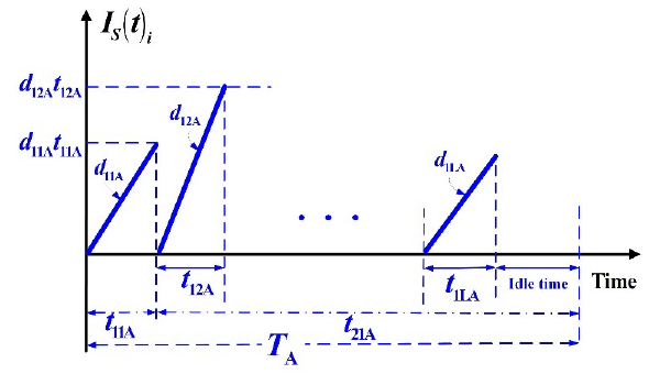
This study explores rotation cycle time and delivery decision for a multi-item producer-retailer integrated system featuring overtime and random scrap. With the aim of reducing production time overtime option is often adopted along with routine manufacturing plan. Consider annual demands λi of L different products must be satisfied by a fabrication system using a rotation cycle rule, that is, during a production cycle each product is replenished one time, in sequence (Figure 1) at an expedited rate P1iA (i.e., overtime is incorporated into the production rate).
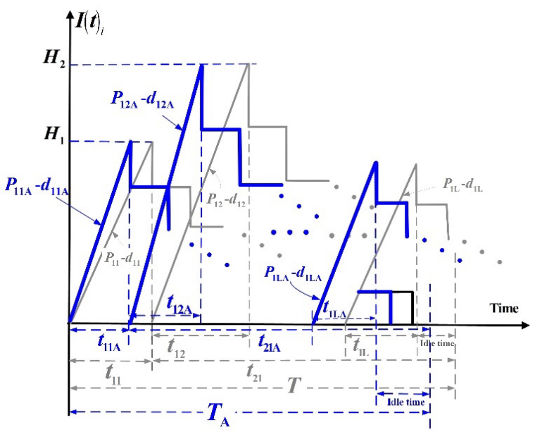
Figure 1 Inventory status of perfect product i in this multi-item producer-retailer integrated system featuring overtime and random scrap (in blue) in comparison with the same system without overtime (in grey)
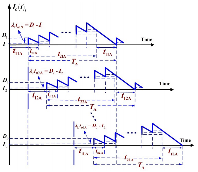
The production processes are not perfect, xi proportion of scraps (where i = 1, 2, …, L) are produced at annual rate d1iA (Figure 2). Due to overtime policy, the following assumptions are made in this study:
where P1i , Ki , and Ci represent the standard production rate, setup and unit production costs; and α1i , α2i, and α3i are the connecting factors between expeditious and standard system variables (see notation list). A few equations can be clearly seen from Figures 1 and 2 as follows:
When uptime ends, fixed size n installments of the completed lot of product i are delivered to retailer at tniA . Inventory status of product i in delivery time t2iA is exhibited in Figure 3 and total inventories during t2iA are calculated as follows (Chiu et al., 2016):
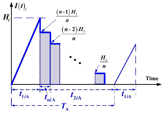
Figure 3 Inventory status of product i in delivery time t2iA in the proposed multi-item producer-retailer integrated system.
(1) For n = 1, total inventories = 0.
(2) For n = 2, total inventories during t2iA are as follows:
(3) For n = 3, total inventories during t2iA become
Therefore, the following general term stands for total inventories of product i during t2iA :
At the retailer side, total stocks of product i can be computed as follows (details please see Appendix A):
3. System cost analysis
Contributors to the system cost TC(TA, n) comprise the following:
(1) Total setup, variable production, and disposal costs for L products.
(2) Total holding costs during uptime and shipping time.
(3) Total fixed and variable delivery costs.
(4) Total holding costs at retailer side.
Therefore, TC(TA, n) is as follows:
Using E[xi] to cope with randomness of xi and replace Equations (4) to (9) in Equation (18), plus further computations, E[TCU(TA, n)] can be obtained:
Or
Where
4. Decision on rotation cycle time and frequency of delivery
The convexity of E[TCU(TA, n)] is first proved by Hessian matrix equations (Rardin, 1998), applying derivatives to Equation (20), we gain the following:
Replace Equations (21) to (23) in Hessian matrix equations plus extra calculations, we found the following:
Because TA, (1 + α2i), and Ki are all positive, so Equation (24) is positive and E[TCU(TA, n)] is strictly convex for all n and TA values other than zero. After proving convexity of E[TCU(TA, n)], next we concurrently locating optimal values of TA* and n*, by setting the following first derivatives of E[TCU(TA, n)] regarding TA and n equal to zero and solving the linear system:
Accordingly, the following TA* and n* are derived with extra derivation efforts:
4.1. Prerequisite capacity condition for the multiproduct fabrication planning
A prerequisite condition (Eq. (29)) for the multiproduct fabrication planning is a guarantee that production equipment has adequate capacity to make L products (Nahmias, 2009). In
addition, another assumption (Eq. (30)) must also be true to avoid the unwanted stock-out situation for each end product i in the batch production planning.
where E[xi] represents the expected scrap rate of product i (see the notation in subsection 2.1.)
4.2. The potential impact of the multiproduct fabrication setup times
The potential impact of the total setup times on the optimal rotation cycle length is as follows. In general, if the sum of setup times is small and can be fitted in the system’s idle time, then the TA* (Eq. (27)) remains valid. Otherwise, one should compute the following Tmin (as shown in Eq. (31)) and choose the actual operating cycle length TA from max(TA*, Tmin) to ensure that it can contain setup times (Nahmias, 2009).
5. Numerical illustration
Assuming that five end items are to be produced in a multi-item producer-retailer integrated system featuring overtime and random scrap, and the relating variables used in this system are displayed in Table 1. Firstly, using Equations (27), (28), and (20), one gets TA* = 0.5817, n* = 3, and E[TCU(TA*, n*)] = $2,758,443. The detailed investigative results on the impacts of differences in
Table 1 The relating variables used in the numerical illustration.
| Item # | xi | λi | P1i | α1i | P1iA | Ci | α3i | CiA | Ki | α2i | CSi | hi | K1i | CTi | h2i | KiA |
|---|---|---|---|---|---|---|---|---|---|---|---|---|---|---|---|---|
| 1 | 5% | 3000 | 58000 | 0.30 | 75400 | 80 | 0.15 | 92 | 10000 | 0.06 | 20 | 10 | 2300 | 0.1 | 50 | 10600 |
| 2 | 10% | 3200 | 59000 | 0.40 | 82600 | 90 | 0.20 | 108 | 11000 | 0.08 | 25 | 15 | 2400 | 0.2 | 55 | 11880 |
| 3 | 15% | 3400 | 60000 | 0.50 | 90000 | 100 | 0.25 | 125 | 12000 | 0.10 | 30 | 20 | 2500 | 0.3 | 60 | 13200 |
| 4 | 20% | 3600 | 61000 | 0.60 | 97600 | 110 | 0.30 | 143 | 13000 | 0.12 | 35 | 25 | 2600 | 0.4 | 65 | 14560 |
| 5 | 25% | 3800 | 62000 | 0.70 | 105400 | 120 | 0.35 | 162 | 14000 | 0.14 | 40 | 30 | 2700 | 0.5 | 70 | 15960 |
Table 2 The impacts of differences in
|
|
n* | TA* | E[TCU(TA*, n*)] [A] | % increase | Total variable production cost [B] | % [B]/ [A] | % increase | Total quality cost [C] | % [C]/ [A] | Sum of delivery cost | Sum of utilization | % decline |
|
|
|---|---|---|---|---|---|---|---|---|---|---|---|---|---|---|
| 0.00 | 3 | 0.5566 | $2,283,398 | - | $1,720,000 | 75.33% | - | $209,047 | 9.16% | $72,673 | 0.3070 | - | 0.00 | 0.00 |
| 0.10 | 3 | 0.5622 | $2,378,103 | 4.15% | $1,813,901 | 76.28% | 5.46% | $208,941 | 8.79% | $72,007 | 0.2791 | -9.09% | 0.02 | 0.05 |
| 0.20 | 3 | 0.5674 | $2,473,000 | 8.30% | $1,907,802 | 77.15% | 10.92% | $208,852 | 8.45% | $71,393 | 0.2559 | -16.67% | 0.04 | 0.10 |
| 0.30 | 3 | 0.5723 | $2,568,043 | 12.47% | $2,001,703 | 77.95% | 16.38% | $208,777 | 8.13% | $70,820 | 0.2362 | -23.08% | 0.06 | 0.15 |
| 0.40 | 3 | 0.5771 | $2,663,199 | 16.63% | $2,095,604 | 78.69% | 21.84% | $208,712 | 7.84% | $70,281 | 0.2193 | -28.57% | 0.08 | 0.20 |
| 0.50 | 3 | 0.5817 | $2,758,443 | 20.80% | $2,189,506 | 79.37% | 27.30% | $208,655 | 7.56% | $69,771 | 0.2047 | -33.33% | 0.10 | 0.25 |
| 0.60 | 3 | 0.5861 | $2,853,758 | 24.98% | $2,283,407 | 80.01% | 32.76% | $208,605 | 7.31% | $69,286 | 0.1919 | -37.50% | 0.12 | 0.30 |
| 0.70 | 3 | 0.5904 | $2,949,128 | 29.16% | $2,377,308 | 80.61% | 38.22% | $208,561 | 7.07% | $68,821 | 0.1806 | -41.18% | 0.14 | 0.35 |
| 0.80 | 3 | 0.5945 | $3,044,544 | 33.33% | $2,471,209 | 81.17% | 43.67% | $208,522 | 6.85% | $68,374 | 0.1706 | -44.44% | 0.16 | 0.40 |
| 0.90 | 3 | 0.5986 | $3,139,996 | 37.51% | $2,565,110 | 81.69% | 49.13% | $208,486 | 6.64% | $67,944 | 0.1616 | -47.37% | 0.18 | 0.45 |
| 1.00 | 3 | 0.6026 | $3,235,478 | 41.70% | $2,659,011 | 82.18% | 54.59% | $208,455 | 6.44% | $67,528 | 0.1535 | -50.00% | 0.20 | 0.50 |
| 1.10 | 3 | 0.6065 | $3,330,985 | 45.88% | $2,752,912 | 82.65% | 60.05% | $208,426 | 6.26% | $67,125 | 0.1462 | -52.38% | 0.22 | 0.55 |
| 1.20 | 3 | 0.6104 | $3,426,510 | 50.06% | $2,846,813 | 83.08% | 65.51% | $208,399 | 6.08% | $66,735 | 0.1396 | -54.55% | 0.24 | 0.60 |
| 1.30 | 3 | 0.6142 | $3,522,052 | 54.25% | $2,940,714 | 83.49% | 70.97% | $208,375 | 5.92% | $66,355 | 0.1335 | -56.52% | 0.26 | 0.65 |
| 1.40 | 3 | 0.6179 | $3,617,606 | 58.43% | $3,034,616 | 83.88% | 76.43% | $208,353 | 5.76% | $65,985 | 0.1279 | -58.33% | 0.28 | 0.70 |
| 1.50 | 3 | 0.6216 | $3,713,171 | 62.62% | $3,128,517 | 84.25% | 81.89% | $208,332 | 5.61% | $65,624 | 0.1228 | -60.00% | 0.30 | 0.75 |
| 1.60 | 3 | 0.6253 | $3,808,744 | 66.80% | $3,222,418 | 84.61% | 87.35% | $208,313 | 5.47% | $65,273 | 0.1181 | -61.54% | 0.32 | 0.80 |
| 1.70 | 3 | 0.6289 | $3,904,323 | 70.99% | $3,316,319 | 84.94% | 92.81% | $208,296 | 5.34% | $64,929 | 0.1137 | -62.96% | 0.34 | 0.85 |
| 1.80 | 3 | 0.6324 | $3,999,907 | 75.17% | $3,410,220 | 85.26% | 98.27% | $208,280 | 5.21% | $64,593 | 0.1097 | -64.29% | 0.36 | 0.90 |
| 1.90 | 3 | 0.6360 | $4,095,494 | 79.36% | $3,504,121 | 85.56% | 103.73% | $208,264 | 5.09% | $64,265 | 0.1059 | -65.52% | 0.38 | 0.95 |
| 2.00 | 4 | 0.7053 | $4,191,061 | 83.54% | $3,598,022 | 85.85% | 109.19% | $208,301 | 4.97% | $76,192 | 0.1023 | -66.67% | 0.40 | 1.00 |
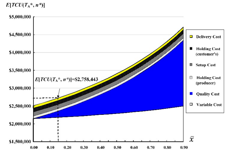
Examining the random scrap factor of the proposed multi-item producer-retailer integrated system, from Table 2, we find out that sum of quality cost is $208,655 (or about 7.56% of E[TCU(TA*, n*)]); besides, the outcomes of examination on the impacts of variations in mean scrap rate x on the system performances, especially on E[TCU(TA*, n*)] and its associated cost factors are shown in Figure 4. It indicates that E[TCU(TA*, n*)] raises significantly, as average scrap rate x goes up; and major contributor to the cost increase is the quality cost, it boosts up drastically, as average x rises. It also confirms that at average x = 0.15, E[TCU(TA*, n*)] = $2,758,443.
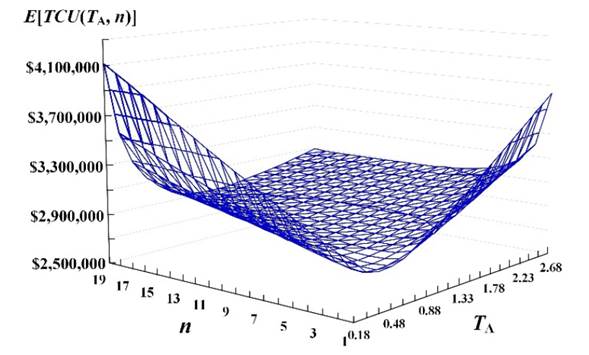
Figure 5 depicts the investigative results on joint impacts of deviations in number of shipments per cycle n and rotation cycle time TA on E[TCU(TA, n)]. It exposes that E[TCU(TA, n)] notably increases, as both TA and n depart from optimal points (i.e., TA* = 0.5817 and n* = 3).
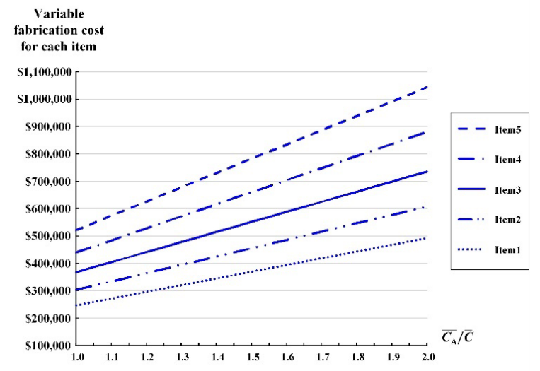
The influence of differences in the ratio of mean overtime unit cost over average ratio of
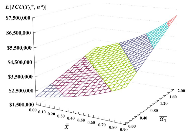
Figure 7 illustrates exploratory results on joint influence of variations in mean scrap rate and mean overtime added proportion of production rate α1 on E[TCU(TA*, n*)]. It shows that E[TCU(TA*, n*)] radically raises, as both
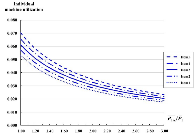
Figure 8 depicts analytical effects of variations in ratio of mean overtime expedited production rate over mean standard rate
On the contrary, Figure 9 shows exploratory outcome on the effect of deviations in
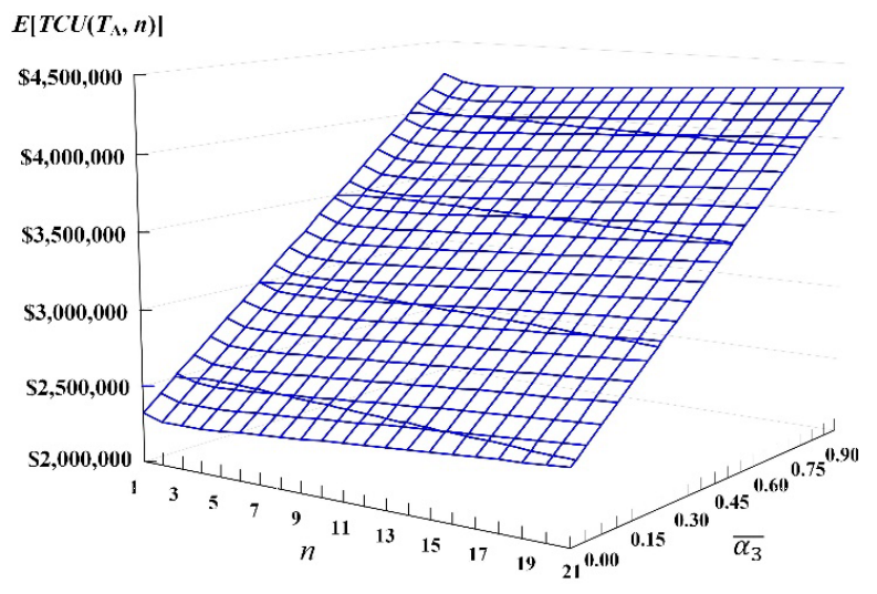
Figure 10 presents the joint influences of changes in n and average overtime unit cost connecting factor
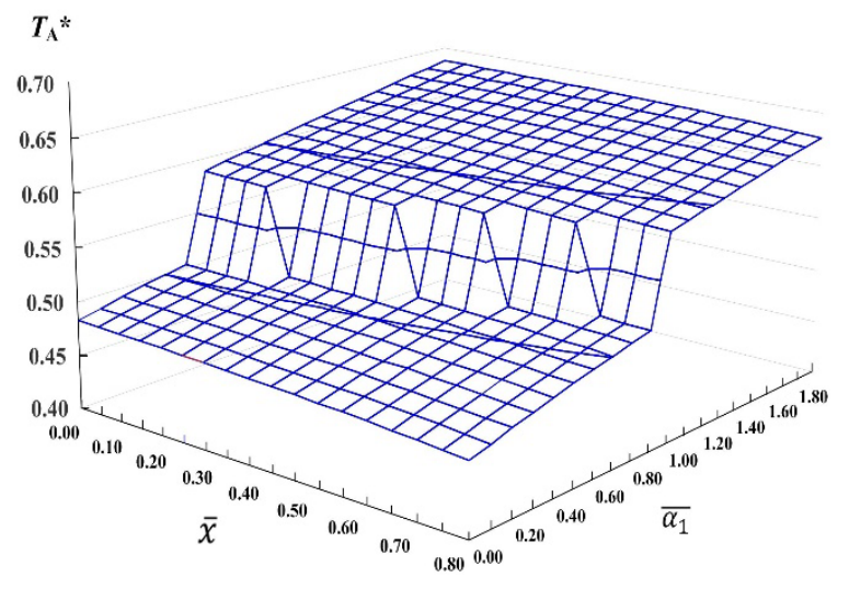
Lastly, further research outcomes on the combined effects of changes in
6. Conclusions
The present study solves the rotation cycle length and delivery decision for a multiproduct producer-retailer integrated system featuring overtime and random scrap. Mathematical modeling and the Hessian matrix equations were applied to tackle the problem and determine the most economic stock refilling and shipping polices. Diverse important system information was revealed that can support managerial decision makings, which includes individual and combined influences of variations in particular system factor(s) (such as overtime related parameters and random scrap rate) on the specific system performance (refer to Figures 4 to 11). Without this profound study, essential system information will remain be concealed. Further investigation on issues of repairing defect items will be an interesting direction for future study.


 nueva página del texto (beta)

