1. Introduction

Clustering is a data mining algorithm whose goal is the grouping of objects. Objects that are similar to each other should belong to the same cluster, and objects that are different from each other should belong to different clusters. There are several clustering algorithms in the literature, for example, partitioning methods, hierarchical methods, density-based method, the neural network-based method and the grid method, graph theory-based method, fuzzy methods. The disadvantage of clustering algorithms is that the algorithms also expect a cluster number as input. The optimal number of clusters can often not be determined by the user, therefore, an algorithm is needed to help the user determine the cluster number. In this paper, we present a representation mode and its evaluation by which the algorithms themselves determine the optimal cluster number. The article is structured as follows: Section 2 contains a brief introduction of clustering algorithms and literature review. Section 3 contains the traditional clustering algorithms, section 4 includes a cluster validation index (Silhouette index). Section 5 contains the construction algorithms, which are the followings: Nearest Neighbor, Nearest Insertion, Cheapest Insertion, Arbitrary Insertion, Farthest Insertion, Greedy. Section 6 includes the improvement algorithms, such as Genetic algorithm, Tabu Search and Particle Swarm Optimization. After that our representation and evaluation is detailed. In section 8 test results are detailed. After that conclusion remarks are made.

2. Clustering

Clustering is a widely used technique for grouping of elements. If two elements are similar, then belong to the same cluster. If they are different, they belong to different clusters. Optimal clustering is a difficult task because there are many ways to group a dataset.

There are lots of types of clustering algorithms, for example (^{Xu & Wunsch, 2005}):

- Partitioning methods: elements are divided into k groups. Each group contains at least one element. After an initial clustering, a re-partitioning follows. At this point, the individual points may be placed in other clusters. The process ends when the elements move slightly (clustering changes only slightly). For example K-Means, Partitioning Around Medoid (PAM)

- Hierarchical methods: clusters can be represented by a dendrogram. There are two main methods of hierarchical clustering: the divisive and the agglomerative methods. The agglomerative methods are Single linkage, complete linkage, group average linkage, median linkage, centroid linkage, Ward’s method etc. The divisive methods are divisive analysis (DIANA), monothetic analysis (MONA).

- Other clustering methods include the density-based method, the neural network-based method and the grid method, graph theory-based method, fuzzy methods.

Some publications have been published in recent years that using metaheuristic algorithms for clustering. The Fast Genetic K-means Clustering Algorithm (^{Lu et al.,2004}) combines the K-Means algorithm and the Genetic Algorithm. The algorithm applies the mutation, selection and crossover techniques (based on the Genetic Algorithm) and also has a K-Means operator. The K-Means operator (one step of the classical K-means algorithm) is the following: the elements are re-partitioned based to the closest cluster centroid. Another clustering analysis with the Genetic Algorithm is introduced in paper (^{Hruschka & Ebecken, 2003}), where also the classical genetic operators are used. The objective function is based on the Average Silhouette Width. The author of paper (^{Maulik & Bandyopadhyay, 2000}) is also used the Genetic Algorithm for the clustering of a data object. The objective function is the minimization of the distance of the objects to their cluster centroids. Their fitness calculation is the following: clusters are formed according to the centers encoded in the chromosome, after the clustering, the cluster centers will be the mean points of the respective clusters. Over the years many crossover and mutation techniques are developed to the Clustering Genetic Algorithm, for example, the one-point mutation, biased one-point mutation, which change the value of a center randomly picked (^{Kudova, 2007}). The K-means mutation, which performs several steps of the k-means algorithm. (^{Kudova, 2007}). The cluster addition and cluster removal modify the number of clusters (adds one center chosen randomly from the data set and deletes one randomly chosen center). (^{Kudova, 2007}) For the fitness function in paper (^{Kudova, 2007}) also the Silhouette is used.

Over the years the Particle Swarm Optimization (PSO) is also applied to clustering data. (^{Li & Yang, 2009}). The PSO is applied with Hierarchical Clustering method, called CPSO Algorithm. A hybrid K-Means PSO algorithm is applied in paper (^{Van der Merwe & Engelbrecht, 2003}). In this case, the result of the K-Means algorithm is improved with the PSO algorithm. The objective function of the PSO algorithm is based on the sum of the average distance of the object to their cluster centroids. In paper (^{Chen & Ye, 2012}) also the PSO algorithm is applied to the clustering of the dataset. In this paper the encoding is also presented, which is the following: the string of the particle contains the cluster centers (in the paper the x and y coordinates of the cluster centroids).

In the case of applying the Ant Colony Optimization (ACO) to clustering data objects, the objective function can be also the minimization of the distance between the cluster elements and the centroids. (^{Runkler, 2005}) The representation of the solution can be a string, which elements are numbers. The numbers indicate the cluster-object assignment. If the string is for example 2,1,3,1, it means, that the first object belongs to cluster 2, the second object belongs to cluster 1, the third object belongs to cluster 3, and the fourth object belongs to cluster 1. (^{Shelokar et al., 2004})

In paper (^{Osman & Christofides, 1994}) the objective function of the Simulated Annealing algorithm is the minimization of the sum of distances between the clusters. The Capacitated Clustering Problem (CCP) is also solved with the Simulated Annealing algorithm. In the case of CCP, each object has a weight, and each cluster has a given capacity which must not be exceeded by the total weight of objects in the cluster.

Cluster Analysis with K-Modes and K-Prototype Algorithms in presented in (^{Madhuri et al., 2014}). The authors used Iris Data Set and Cholesterol Data Set for Incremental k-Means, Contact-Lens Data Set and Post-operative Data Set for Modified k-Modes, Blood Information Data Set and Weather Data Set for k-Prototypes .

Automatic clustering with Teaching Learning-Based Optimization (TLBO) is presented in paper (^{Murty, Naik et al., 2014}). The efficiency of the TLBO is compared also with Particle Swarm Optimization (PSO), Differential Evolution (DE). The efficiency of the algorithms is compared with the following benchmark datasets: Iris Data, Wine Data, Breast Cancer Data, Glass Data and Vowel Data.

The purpose of cluster validation indices is to compare individual clusters with each other considering certain aspects. Several such indices have been published, but these indices are not suitable for data sets of any size, density, shape. The authors of (^{Murty, Murthy et al., 2014}) have developed a validation index (Homogeneity Separateness) that is effective for clusters of any shape, size, and density. Some clustering problems and the algorithms that solve it are illustrated in Table 1.

3. Traditional clustering algorithms

In this section, the applied traditional clustering algorithms are presented based on the literature.

3.1. K-Means

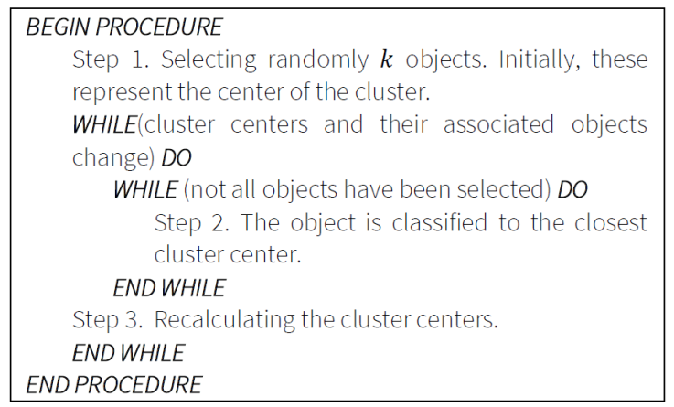
This procedure belongs to a group of partitioning methods. First, the elements are clustered and then the elements move from the initial clusters to improve the quality of the clustering. The algorithm uses the SSE function. Here, the number of clusters (k) must be specified. (^{Wagstaff et al., 2001}) Figure 1 illustrates the psedo code of the K-Means algorithm.

Figure 1 The pseudo code of the K-Means method (^{Wagstaff et al., 2001}). 

EC=∑i=1k∑u∈Cid(u,rCi)2 (1)

4. Hierarchical methods

These algorithms organize the clusters into a hierarchical data structure. There are two types of algorithms: bottom-up and top-down. At the bottom-up, each element is initially a cluster, and then each cluster is merged into a single cluster. The top-down procedure is just the opposite. Here at first, there is a single cluster that contains all the elements, and we continually divide the clusters. At the end of the procedure, each element means a separate cluster. The following hierarchical clustering is applied in this paper: (^{Murtagh, 1983}; ^{Olson, 1995})

Single Linkage: The distance of the two clusters is the distance between the nearest objects of the two clusters:

Complete Linkage: the distance of two clusters is the distance between the farthest objects of two clusters:

Average method: the distance of two clusters is the quotient of the sum of the distances between the objects of two clusters and the number of clusters:

Centroid method: the distance of two clusters will be the distance of the center of two clusters:

Ward method: merging the two clusters that cause the least-squares error increase:

5. Cluster validation index

Let {A} be a partitioning, i is the index of the data point, and Ai denotes the container cluster of element i. The silhouette index of the object i is (^{Wang & Xu, 2019}):

where, -1≤s(i)≤1.

a(i) is the average distance between the object i and other objects in cluster Ai,b(i) is the average distance between the object i and all other cluster elements (except elements in cluster A). Thus a(i) denotes compactness and b(i) denotes separation.

- If s(i) is large (close to 1) then the inner (within the cluster) difference is much smaller than the smallest outer cluster difference. Hence, we can say that object i . is well grouped.

- If s(i)= 0, or very close to zero, then a(i) and b(i) are nearly equal, then object i may belong to cluster A or B .

- If s(i) is close to -1, then a(i) is much greater than b(i). This means that cluster B would be a better choice than cluster A .

With the silhouette method, we can measure the efficiency of the whole cluster result. For each element, s(i) should be calculated and the results should be averaged.

The following conclusions can be made from the average silhouette:

- 0.5 or higher value: good clustering

- 0.25-0.5: the clustering method is good, but some object should be moved to another cluster

- Less than 0.25: Not good clustering

Thus, the higher the average silhouette, the better the clustering.

Therefore, the objective function of our improvement algorithms is the average silhouette value.

6. Tour-based construction clustering algorithm

Behind this approach is the shortest route path tour connects neighboring elements. The edge distance is usually small, it connects elements from the same cluster, but the length is large if the edge connects two distinct clusters. Testing the distance of the connecting edges of the optimal tour the edges with high lengths denote existence of the separate clusters.

The construction algorithms construct one possible solution. Running time is relatively low. These algorithms always take locally the best steps. Most of the time, the global optimum is not achieved by their exclusive usage. The construction algorithms are based on the Traveling Salesman Problem algorithms.

6.1. Nearest neighbor

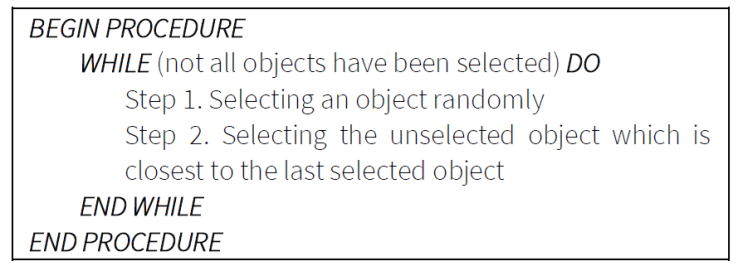
The algorithm always selects the unselected object that is closest to the last selected object. The algorithm is fast and simple. Figure 2 illustrates the pseudo code of the Nearest Neighbor algorithm.

Figure 2 The pseudo code of the Nearest Neighbor algorithm (^{Nilsson, 2003}). 

6.2. Nearest insertion

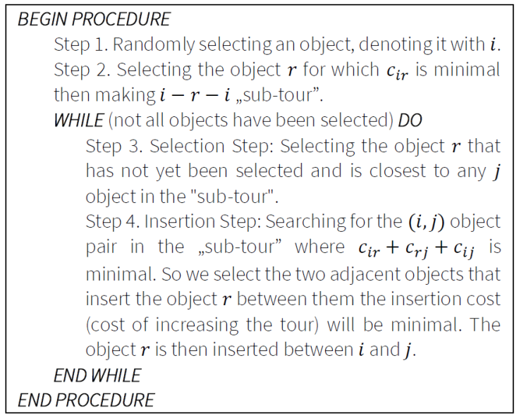
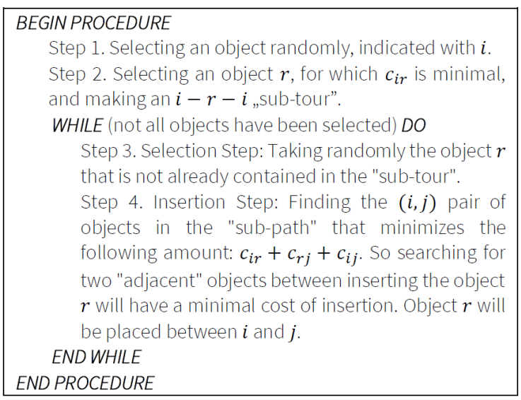
The algorithm belongs to the group of insertion heuristics. The algorithm always selects the unselected object that is closest to the "tour". The distance between the "tour" and an object is interpreted by the algorithm as the minimum distance between the objects in the tour. The pseudo code of the Nearest Insertion algorithm is illustrated in Figure 3.

Figure 3 The pseudo code of the Nearest Insertion algorithm (^{Golden et al., 1980}). 

6.3. Cheapest insertion

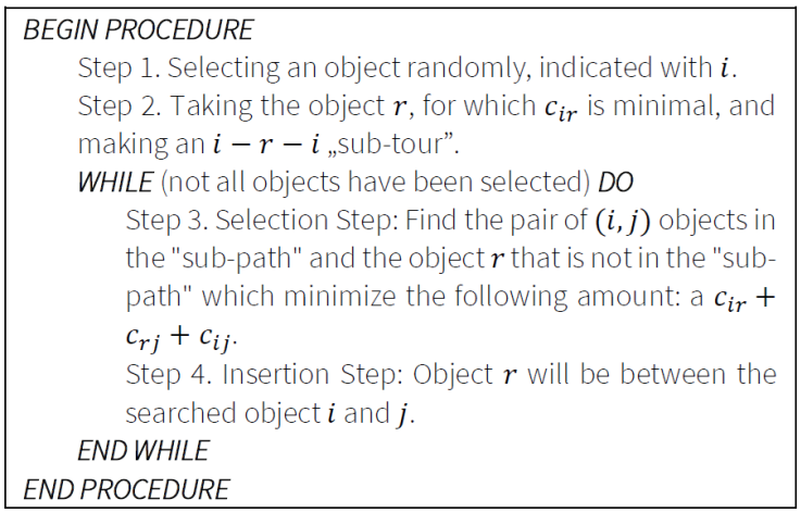
This algorithm also belongs to the group of insertion heuristics. The algorithm always selects the object with the least "insertion cost" into the “tour". Figure 4 illustrates the pseudo code of the Cheapest Insertion.

Figure 4 The pseudo code of the Cheapest Insertion algorithm (^{Golden et al., 1980}). 

6.4. Arbitrary insertion

This algorithm also belongs to the group of Insertion Heuristics. The algorithm randomly selects the next object to be inserted into the "tour". Figure 5 presents the presudo code of the Arbitrary Insertion algorithm.

Figure 5 The pseudo code of the Arbitrary Insertion algorithm (^{Rosenkrantz et al., 1974}). 

6.5. Farthest insertion

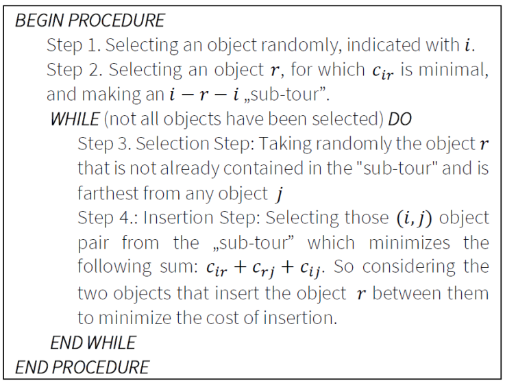
This algorithm also belongs to the Insertion Heuristics group. The object that is farthest from the other objects is selected by the algorithm. Figure 6 illustrates the pseudo code of the Farthest Insertion algorithm.

Figure 6 The pseudo code of the Farthest Insertion algorithm (^{Golden et al., 1980}). 

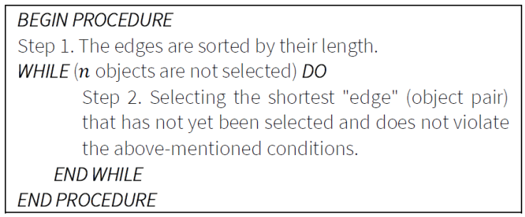
6.6. Greedy

Each object builds the order from "edges" (pairs of objects) so that it always selects the shortest "edge" that has not yet been selected and does not form n vertex circles (n indicates the number of objects). Also, the degree of the “edge” should not be more than two. The pseudo code of the Greedy algorithm is illustrated in Figure 7.

Figure 7 The pseudo code of the Greedy algorithm (^{Nilsson, 2003}). 

7. Tour improvement-based clustering algorithm

Behind this approach is also the fact, that the shortest route path tour connects neighboring elements. This method tries to improve an existing path by rearranging the order of the elements iteratively. Their running time can be high, and their exclusive usage does not lead to the global optimum in most of the cases.

7.1. Genetic algorithm

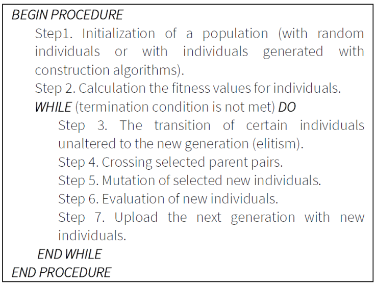
The algorithm models natural processes (evolution). The algorithm works with a population of solutions. The population consists of individuals. (^{Milano & Koumoutsakos, 2002}) Individuals have fitness values. Usually, an individual with better fitness value is better against other individuals. The pseudo code of the Genetic Algorithm is presented in Figure 8.

Figure 8 The pseudo code of the Genetic Algorithm (^{Whitley, 1994}). 

The first step is the initialization of the population. This process is usually done with randomly generated individuals. Then the fitness values of the individuals are calculated. Then the next population is created in a cycle while the termination condition is not met. The termination condition may be to achieve a certain iteration number or runtime. The next population is created by moving certain individuals unchanged, which is called elitism. The other elements are created with crossover and mutation techniques. We have used the 2-opt (^{Wu et al., 2007}) as mutation, and the Partially Matched Crossover (PMX) (^{Lazzerini & Marcelloni, 2000}) (^{Starkweather et al., 1991}), the Order Crossover (OX) (^{Starkweather et al., 1991}), and the Cycle Crossover (CX) (Starkweather et al., 1991) as crossover operators.

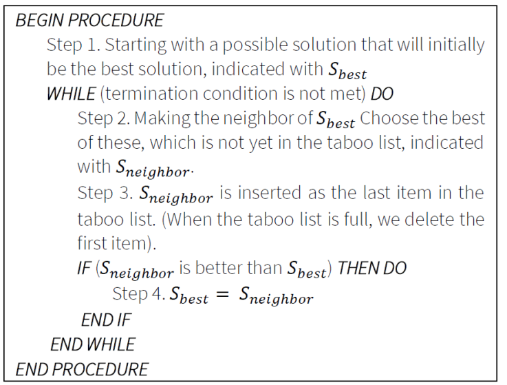
7.2. Tabu search (TS)

The algorithm maintains a taboo list containing the results of the last few steps. In the process, we can only take the neighbor of the current solution that is not in the taboo list. The taboo list must be changed at each iteration. If you add a new item, you must delete the first item from the beginning if the list is already full. (^{Glover & Laguna, 1998}) The pseudo code of the Tabu Search is illustrated in Figure 9.

Figure 9 The pseudo code of the Tabu Search (^{Glover & Laguna, 1998}). 

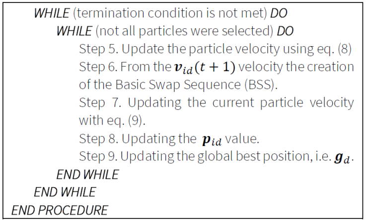
7.3. Particle Swarm Optimization

It maintains a population of possible solutions. The particles move through the search space using a simple mathematical formula. Particle movement is determined by the best search space positions found (the best position of the particle and the best position on the particle - best of all).

The algorithms use the following formulas:

1. Particle velocity updating formula:

vidt+1=vidt⊕αpid-xidt⊕β(gd-xid(t)) (8)

Current particle velocity updating:

xid(t+1)=xid(t)+vid(t+1) (9)

where the following notations are used:

•  vid(t): the new velocity (swap sequence).

• pid-xid(t): the difference between the best and current particle position (Basic Swap Sequence - BSS (^{Wang et al., 2003}).

• gd-xid(t): the difference between the globally best particle position and the current position of a given particle (Basic Swap Sequence - BSS (^{Wang et al., 2003}).

• α,β∈ [0,1] are random numbers. The ⊕ operation (^{Wang et al., 2003}) is the sequential execution of the swap sequences. Figure 10 illustrates the pseudo code of the Particle Swarm Optimization.

Figure 10 The pseudo code of the Particle Swarm Optimization (^{Wang et al., 2003}). 

8. Representation of clustering task, its evaluation, objective function

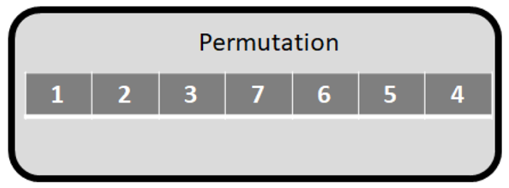
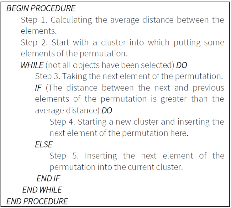
When applying construction and improvement algorithms for solving the clustering problem, we need to use a representation mode. In this paper permutation representation (mapping vector) is applied (Figure 11). The elements of the mapping vector are the individual objects. The objective function (of the improvement heuristics i.e., PSO, GA, TS) is to maximize the Silhouette value. The evaluation of the mapping vector is illustrated in Figure 12.

Figure 11 The permutation (mapping vector) representation. 

Figure 12 The evaluation of the mapping vector. 

9. Test results

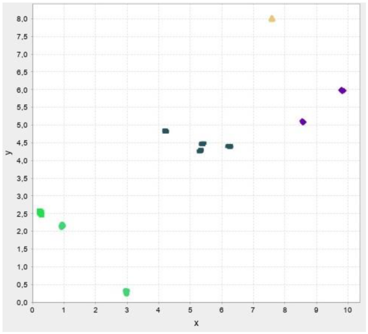
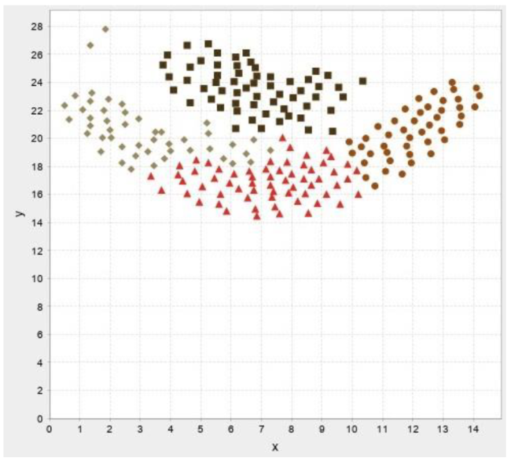
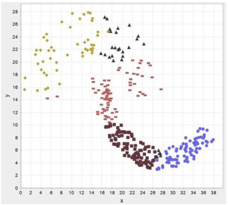
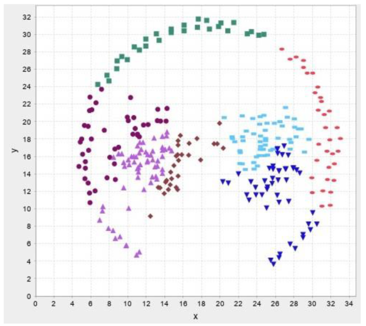
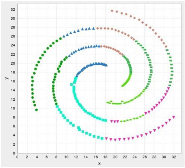
In this section, the test results are presented. First, test results for our own data then results for benchmark datasets are presented. The abbreviations and their meaning is presented in Table 2. Figure 13-17 illustrates the test result of the algorithms.

Figure 13 The result of average linkage for our data. 

Figure 14 The result of complete linkage for flame data. 

Figure 15 The result of K-Means for Jain data. 

Figure 16 The result of Arbitrary Insertion for Pathbased data. 

Figure 17 The result of Arbitrary Insertion for Spiral data. 

In Table 3-7 the N means the number of objects and k means the optimal number of clusters. In these tables the average values of 10 test runs are detailed. Table 8 present the summary of the test results.

In the following test results of the benchmark datasets from (^{Fränti & Sieranoja, 2014}) is presented.

The test results show that despite the failure to reach the desired number of clusters, the silhouette values are high, so the implemented algorithms cluster relatively well. We do not recommend using improvement algorithms due to their high running time, we only recommend modified versions of construction algorithms and traditional clustering procedures.

10. Conclusion

In this article different tour-based clustering algorithms are compared with the classical methods and analyzed. After the literature review the traditional clustering algorithms (K-Means, Hierarchical Methods) are presented, then the Silhouette index to measure the quality of the clustering result. After that construction algorithms and improvement algorithms are detailed. Then our cluster representation technique and evaluation is described. After that test results are presented. In the test we have implemented and analyzed the main clustering methods and the tour construction and tour improvement methods. The comparison test performed on self-generated dataset and several clustering benchmark test: Flame, Jain, Pathbased and Spiral. Based on the test results the traditional clustering algorithms and the construction algorithms have efficiency in partitioning datasets with our representation and evaluation technique.