


 nueva página del texto (beta)
 Inglés (pdf)
 Artículo en XML
 Referencias del artículo
 Enviar artículo por email
 Citado por SciELO
  Similares en
SciELO
Similares en
SciELO 
 Permalink
1. Introduction
Direct current (DC) motors are used in electromechanical systems that require precise positioning, especially in robotic applications (Aravind et al., 2017). Some reasons for that choice are discussed in (Durdu & Dursun, 2018), where it is highlighted their high efficiency, satisfactory performance, and simple control procedures. Thus, several studies are presented in the literature about the angular position control of DC motors: Linear Quadratic Gaussian (LQG) control with Extended Kalman Filter (EKF) (Aravind et al., 2017); sliding mode control with variable structure (Durdu & Dursun, 2018; Qureshi et al., 2016); Proportional-Integrative-Derivative (PID) control with friction compensation (Maung et al., 2018); PID control considering the presence of Stribeck friction (Tumbuan et al., 2019); PID control where its parameters are tuned by genetic algorithm (Thomas & Poongodi, 2009; Tiwari et al., 2018); a comparison study between PID control strategies with either genetic algorithms or fuzzy self-tuning (Flores-Morán et al., 2018); a comparative analysis among the performance obtained from PID and fuzzy controllers, aiming the position control of electromechanical actuators coupled to DC motors and to a 6 Degrees Of Freedom (DOF) platform (Breganon et al., 2019), position control using PID and Linear Quadratic Regulator (LQR) (Chotai & Narwekar, 2017).
A comprehensive study of pole placement for DC motor’s control using different state feedback control techniques, where the performance of the state feedback, feed-forward gain with state feedback, and integral control with state feedback controller are investigated, is presented in (Ahmad et al., 2018). Moreover, the design and implementation of a position controller through state feedback for a rotary platform driven by a DC motor are shown in (Carlos et al., 2017).
An advantage of state feedback control is the possibility to place the system’s poles of the closed-loop system in order to achieve a desired performance, since the system has the controllability characteristic (Breganon et al., 2020a; Ogata, 2010). However, the state feedback requires the measurement of all state variables from the plant for the control signal calculation, fact that can generate expensive cost in the system instrumentation (due to the use of several sensors) or even make the control implementation unfeasible. To overcome this difficulty, a state observer is a valid option since the system has the observability characteristic (Ogata, 2010).
The use of digital computers in the feedback loop is a trend in the process control, which allows the integration between the plants and supervisory systems. When a digital computer is used in the control loop, it is necessary the use of digital/analog converters inside the loop. This fact can deteriorate the performance of the closed-loop system when these devices are not considered in the control design and/or when the sampling period is excessively long. In order to improve the control performance, in this case, it is possible to make the discretization of the system’s dynamic and then design the controller in discrete time (Franklin et al., 1998). A discrete PI controller to control a DC motor that has a load connected to its axis is show in (Breganon et al., 2020b).
In this sense, this work explores the use of the state feedback with pole placement in association with a state observer to control the angular position of a DC motor coupled on an inertial load. In addition to the simulation results, results from real experiments (bench scale) are also presented to validate the obtained model and the proposed control strategy.
The next sections of this paper are organized as following. In Section 2, the state-space model of a DC motor coupled to an inertial load is described. The experiments and procedures performed to obtain the main parameters of the system’s model (motor + load) are also presented in this section, as well as the discretization of the obtained model. The state feedback control considering an observer in the control loop is addressed in Section 3. In Section 4, the experimental setup and the obtained results are presented. Finally, the main conclusions of this work are discussed in Section 5.
2. Motor’s model
The diagram of a DC motor is illustrated in Figure 1 (Nise, 2011). It can be observed that, once a voltage v(t) is applied on the motor, a current i(t) arises in the armature’s circuit. In the armature’s circuit there is a resistance R a and an inductance L a .

The back electromotive force generated in the armature by the motor’s rotation is proportional to its angular velocity, that is:
Where θ(t) is the angle of the motor’s axis.
Applying the Kirchhoff’s voltage law in the DC motor’s armature loop, and also using Eq. 1, we have
It is known that the torque on the motor’s axis is proportional to the current in the motor’s armature. Using a consistent set of units, this constant is K m , the same constant presents in Eq. 1 (Guo & Mohamed, 2020; Nise, 2011).
The torque developed on the motor’s axis is opposite to that one due to the viscous friction, using the Newton’ Law for rotation, and considering the inertia connected to the motor’s axis (Iswanto et al., 2021; Ma’arif & Setiawan, 2021):
Where b is the coefficient of viscous friction in the motor’s axis,
and J is the moment of inertia coupled to it. We can replace the
current in Eq. 2 by using Eq. 3. From that step and then isolating
where
Using as state variables x
1(t) = θ(t),
x
2(t) =
in which
where
Remark 1. In order to impose constant values to the angular position of
the motor’s axis, the following changing of variables can be considered in Eq. 6: x
N1
(t) = x
1(t) - r, x
N2
(t) = x
2(t) and x
N3
(t) = x
3(t). In this way, if
in which x N (t) = [x N1 (t) x N2 (t) x N3 (t)] T , and then the convergence of x N (t) to zero implies the convergence of x 1(t) to r.
2.1. Parameters’ identification
The blocked rotor test was performed to obtain the value of the armature’s resistance, where the rotor was securely locked while a constant voltage was applied on the motor. In that condition, the electric current is constant, and the back electromotive force is null, because it is proportional to the rotation velocity (Eq. 1), which is also null. The resistance value is obtained from that condition, by means of the relation between the measured voltage and current. v = 0.23 V, i = 0.117 A and R a = v/i = 1.965 Ω.
After this test, knowing the armature’s resistance value, the motor’s torque was
determined through another experiment. Constant values of voltage
v(t), with voltage interval of 1 V within
the voltage spam of the motor, were applied on the motor while the state-steady
armature’s current and the respective axis’ velocities were measured. Next, the
armature’s voltage v
ce
(t) was computed through Kirchhoff’s Law (Eq. 2) with
In these tests, as the motor’s torque is proportional to the current
(τ(t) = K
m
i(t)) and it faces the torque due to the
damping
Table 1 Data from continuous voltage applied on the motor.
| Applied Voltage v(t) [V] | Measured Current i(t) [A] | Back Electromotive Force v ce (t) = v(t) - Ri(t) [V] | Angular Velocity |
Constant K m [N.m / A] | Damping Coefficient b b = i.K m /ω [N.m.s / rad] |
|---|---|---|---|---|---|
| 0.9825 | 0.051 | 0.88224359 | 16.96460033 | 0.052004973 | 0.000155674 |
| 2.068 | 0.057 | 1.955948718 | 37.72005579 | 0.051854343 | 7.82513E-05 |
| 3.066 | 0.061 | 2.94608547 | 56.67433147 | 0.051982712 | 5.57356E-05 |
| 4.121 | 0.064 | 3.995188034 | 77.01090791 | 0.05187821 | 4.30345E-05 |
| 5.061 | 0.067 | 4.929290598 | 95.13789753 | 0.051812062 | 3.64678E-05 |
| 6.059 | 0.071 | 5.91942735 | 114.3539726 | 0.051764073 | 3.21511E-05 |
| 7.054 | 0.074 | 6.908529915 | 133.3082483 | 0.051823724 | 2.87451E-05 |
| 8.067 | 0.08 | 7.909735043 | 152.8908425 | 0.051734525 | 2.70955E-05 |
| 9.018 | 0.081 | 8.858769231 | 171.2167996 | 0.05174007 | 2.44978E-05 |
| 10.024 | 0.085 | 9.856905983 | 190.5899543 | 0.051717867 | 2.30945E-05 |
| 11.04 | 0.09 | 10.86307692 | 210.4867078 | 0.051609325 | 2.21415E-05 |
| 12.1 | 0.095 | 11.91324786 | 231.4306588 | 0.051476533 | 2.12565E-05 |
| Average | 0.051783201 | 2.69312E-05* |
* The average of the damping coefficient values does not consider the first four damping values listed
The armature’s inductance L a was determined from the measurement of the motor’s RMS electric currents due to the alternating voltage magnitude variation. In these tests, the frequency of the alternating voltage was selected close to that one from the Pulse Width Modulation (PWM) used by the controller board. From the data presented in Tables 1 and 2,
in which X L is the inductive reactance and ׀z׀ is the motor’s impedance magnitude. From Eq. 9, the inductance is computed as
where f represents the frequency (in Hz) of the voltage applied to the motor.
Table 2 Data from alternating voltage applied on the motor.
| RMS Voltage Value v ef (t) [V] | RMS Measured Current i ef(t) [A] | Frequency f [Hz] | Impedance Magnitude |
Inductive Reactance X L (Eq. 9) [Ω] | Inductance L (Eq. 10) [H] |
|---|---|---|---|---|---|
| 1.352 | 0.1 | 4966 | 13.52 | 13.37632174 | 0.000428697 |
| 0.1 | 0.0074 | 4985 | 13.51351351 | 13.36976555 | 0.000426853 |
| 0.219 | 0.01672 | 5045 | 13.09808612 | 12.94972754 | 0.000408526 |
| 0.308 | 0.0233 | 5040 | 13.21888412 | 13.0718966 | 0.000412789 |
| 0.402 | 0.03036 | 5016 | 13.24110672 | 13.09436865 | 0.000415477 |
| 0.5003 | 0.03783 | 4967 | 13.22495374 | 13.22459063 | 0.000423749 |
| 0.5999 | 0.04522 | 4969 | 13.26625387 | 13.26611363 | 0.000424908 |
| 0.708 | 0.05261 | 4971 | 13.45751758 | 13.45737933 | 0.000430861 |
| 0.804 | 0.05992 | 4974 | 13.41789052 | 13.41775186 | 0.000429333 |
| 0.909 | 0.06722 | 4983 | 13.52276108 | 13.5226235 | 0.000431907 |
| 1.001 | 0.07452 | 4982 | 13.43263553 | 13.43249703 | 0.000429114 |
| Average | 0.000423838 |
Moreover, there is an inertial load coupled to the motor. That load consists of a cylinder manufactured with nylon with a centralized hole compatible to the size of the motor’s axis for coupling, and it is linked to an aluminum rod, as shown in Figure 2. The cylinder has external and internal radius of R c1 = 15×10-3 m and R c2 = 3×10⁻³ m, respectively, and mass of m c = 17×10-3 kg. The rod has length of l b = 184.8×10⁻³m and mass of m b = 16.4×10⁻³ kg.

The inertia of the axis’ movement, due to the load shown in Figure 2, can be computed by the sum of inertias of the set of the cylinder and rod together. The inertia related to the cylinder is computed as
while the inertial part related to the rod is calculated by
Finally, from Eqs. 11 and 12, the inertia coupled to the motor is computed as
Using the data from Tables 1 and 2, and J from Eq. 13, the plant consisting of the DC motor coupled to the load (Figure 2) is described by the dynamic Eq. 6, where the matrices A, B and C are given by
2.2. Model discretization
In the control project, a computer is considered as the system’s controller, in which the sampling period T s is constant. Figure 3 illustrates the considered feedback control loop, where D/A and A/D represent the digital to analog and the analog to digital converters, respectively. The plant considered is the motor+load system, which is given by Eqs. 6 and14.
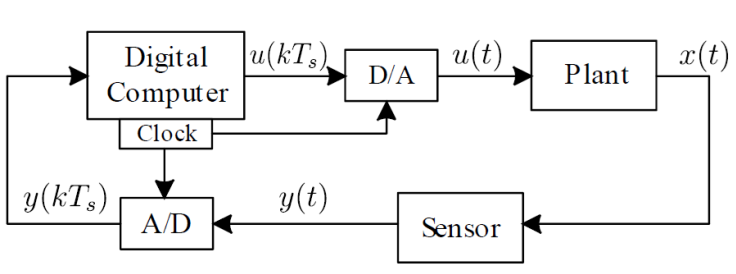
Based on the diagram in Figure 3, a discrete time representation of the plant can be obtained from the response of the system (Eq. 6) in continuous time and then sampling this result according to the period T s , as shown in (Franklin et al., 1998). Using this procedure and considering that the control signal is applied with a Zero Order Holder (ZOH), the plant (Eq. 6) is described in discrete time by
in which the matrices
are computationally calculated. From model Eq. 6 with sampling period T s = 0.02 s and the matrices in Eq. 14, the matrices in Eq. 16 are computed as given by Eq. 17.
Observe that the matrix C remains the same at both continuous and discrete time models.
3. State feedback control with pole placement and state observer
In this work, the state feedback control law is considered in discrete time, and it is described by
where K ∈ ℜ3 is a constant vector such that the closed-loop system has the desired eigenvalues. Considering system (Eq. 15) in closed-loop with the control law (Eq. 18), the resulted closed-loop dynamic is given by
As the closed-loop system’s dynamic is related to the poles in the Z-plane, the gain K in Eq. 18 directly influences the dynamic of the closed-loop system. The design of the gain K can be performed by different ways. One of the possibilities is the use of the Ackerman formula to perform the poles placement of the closed-loop system (Ogata, 2010). It is important to observe that, for that approach, the system must be controllable.
3.1. State observer in the control loop
Observe that the control law described in Eq. 18 allows great flexibility in the control design and leads to obtain the desired characteristics of the closed-loop system. However, this control law requires the measurement of all state variables of the system, it can make the control system more expensive or even make it unfeasible. One solution for this problem consists of using a state observer and then using the control law
where
Defining the observation error as
Thus, if the matrix L is chosen such that the dynamic of Eq. 22 is stable, then
A diagram of the closed-loop system considering a state observer is shown in
Figure 4. Observe that the control law
(Eq. 20) is used to generate
the control signal that is sent to the plant, and it is also used to compute the
estimated state
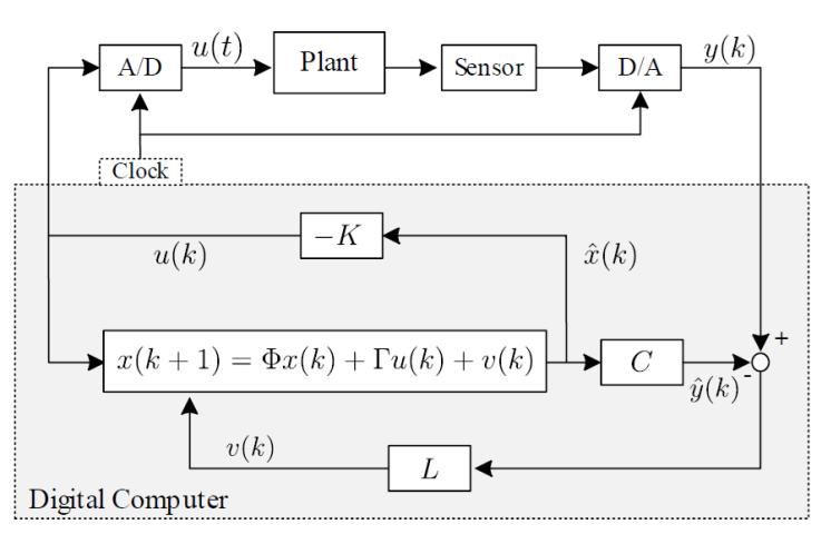
Considering the dynamic in Eq. 15, the control law (Eq. 20) and the observation error (Eq. 22), the closed-loop system is described by
and, by using
Thus, the eigenvalues of the system (Eq. 24) depend on the eigenvalues of the matrices Φ-ΓK and Φ + LC, that is, on the eigenvalues of the systems Eqs. 19 and 22. Consequently, the gain matrices K and L can be independently designed (Ogata, 2010).
In this work, the matrices K and L were designed using the pole placement methodology (Ogata, 2010). The poles chosen for the design of the controller gain K were p 1 = 0.098, p 2 = 0.906+j0.01, and p 3 = 0.906-j0.01 while the poles chosen for the design of the observer gain L were l 1 =0.0101, l 2 =0.0099, and l 3 =0.0097. These values were chosen by trial and error in such a way the closed-loop system could show a response that would be within the limitations of the equipment as well as match the design requirements.
Based on this design, the obtained gains were
and
4. Results and discussions
A Maxon DC motor with a DC voltage source of 12 V and an H bridge for actioning were used for the practical experiments. The considered motor is coupled to an incremental encoder with 500 pulses per revolution, used to measure the angular position of the motor’s axis. The H bridge and the encoder are connected to a data acquisition board from National Instruments®, model PCI-6602, that exchanges data with a computer, whose configuration is: Intel Core 2 Duo E8600 3.33 GHz, with 2 GB of RAM. The control system was implemented via the Matlab/Simulink® software. The experimental setup is shown in Figure 5.

Remark 2. The considered motor has a dead zone of 0.27 V, approximately. In the control implementation, this dead zone was compensated by a function block described by û(t) = sign(u(t)) [׀u(t)׀ + 0.27], where sign (·) is the signal function and u(t) is the control signal given by the controller. Then, after the control signal correction made by this block, û(t) is the control signal sent to the plant.
The control of the motor was performed using the control diagram of Figure 4 with the matrices Φ and Γ given by Eq. 17, C in Eq. 7 and gains in Eqs. 25 and 26. Simulations were also carried out using dynamic Eq. 15 instead of the plant in Figure 4.
In Figures 6 - 10 the main results from the simulations and the experimental tests performed in the bench (Figure 5) are presented.
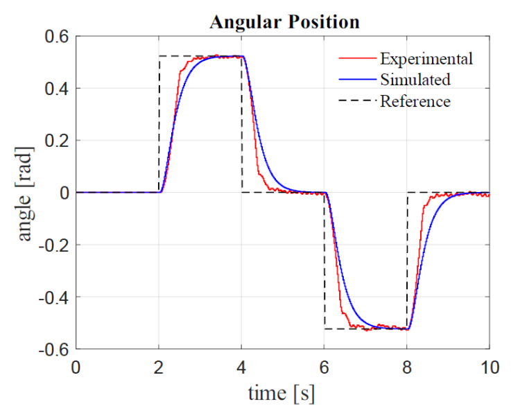

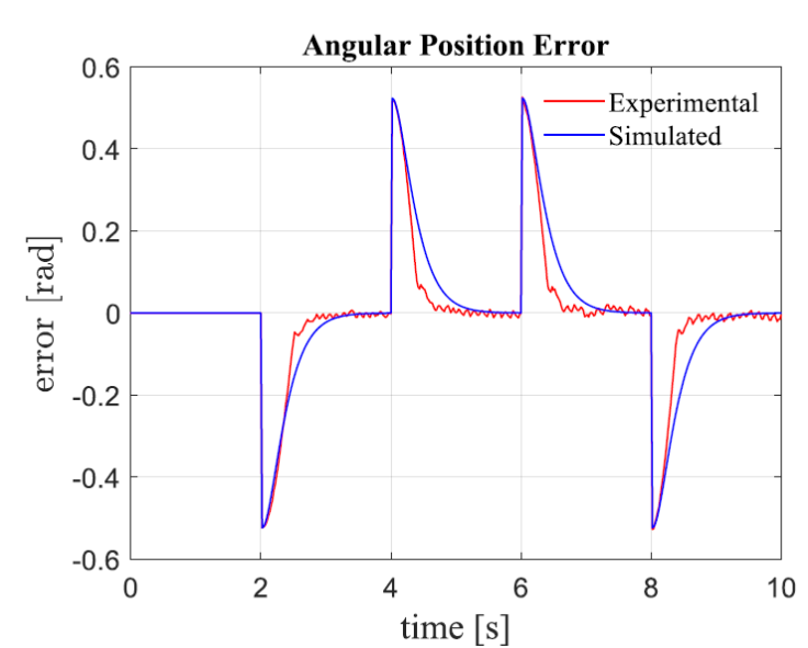
Figure 8 Error between the motor’s axis angle and the reference, obtained from simulation and experimental test.


The results of the controlled system are compared in Figures 6-8, considering a step
reference. At the instant 2 s a step of amplitude
Table 3 System’s Stabilization Time.
| Amplitude of the reference step [rad] | Time of the reference changing [s] | Stabilization Time [s] | |
|---|---|---|---|
| Simulated | Experimental | ||
|
|
2 | 3.78 | 3.36 |
| 0 | 4 | 5.88 | 5.08 |
|
|
6 | 7.86 | 6.96 |
| 0 | 8 | 9.86 | 9.50 |
In these figures (Figures 6-8), it is observed that the results from simulation and experimental tests were similar, validating the mathematical model of the motor. It is noticed that although the control signal is relatively low, as shown in Figure 7, the angular position of the motor’s axis fulfills the project requirements (Figure 6), as well as the error between the angle and the reference (Figure 8), tending to zero in both situations (simulations and experimental tests). The settling time that can be observed in Figure 6, above 1 second, is related with the chosen poles in the design of the controller. Even though it can be considered a slow response, it was adequate to its implementation in the prototype used for the tests.
In addition, the dead zone of the motor and its compensation in the control action are not considering in the simulation. However, the obtained response was appropriate and according to the project requirements, as can be noticed in Figure 6.
In Figures 9 and 10 the state variables estimated by the observer, in simulation (Figure 9) and in the experimental test (Figure 10) are presented, in which x 1(k) is the angular position, x 2(k) is the angular velocity and, finally, x 3(k) is the angular acceleration. It is interesting to observe that the state variables estimated during experimental tests present measurement noises in the state variable x 1(k), which are amplified in the estimation process.
5. Conclusions
This work presented a procedure to mathematically model a DC motor with a load coupled to its axis, in continuous and discrete time. The system’s parameters were detailed, and its values are obtained by means of experiments described in this paper. After the modeling step, a digital control strategy based on state feedback, using a state observer, was considered to control the angular position of the motor’s axis. The gains in this strategy were designed by means of the pole placement technique. The obtained results, both in simulation and in the performed experimental tests, showed that the mathematical model of the motor is valid, as well as the applied control scheme provides satisfactory results. For future works, we intent to explore more control strategies, besides complement the experimental setup with other type of loads to be coupled to the motor axis.

