Highlights:
NOX, O3, CO, PM10 and PM2.5 were analyzed in Mexico City Metropolitan Area (MCMA)
Spatio-temporal dynamics varied among pollutants in MCMA.
Pollutant concentrations decreased in the periods studied.
NOX had the largest decrease (-1.28 ppb∙yr-1), and CO had the smallest change (-0.12 ppm∙yr-1).
Support Vector Machine had the best fit for pollutant interpolation.
Introduction
Air pollutants are one of the main problems in large cities, because of high population density, increased urbanization, transportation and industrialization (Guzmán-Morales et al., 2011). The Mexico City Metropolitan Area (MCMA) is one of the most populated regions in the world; according to the latest population and housing census, the area has 20.1 million inhabitants and an average monthly movement of more than 46 million cars (National Institute of Statistics and Geography [INEGI], 2020, 2022). This emphasizes the importance of the study and measurement of air pollutants in the urban area, especially in a spatial context (Camarillo et al., 2014).
The MCMA has unfavorable conditions for air ventilation, due to the mountains surrounding the basin of the Valley of Mexico, a situation that complicates the dispersion of pollutants (Barrera Huertas et al., 2019). The MCMA covers an area of 4 726.4 km2 and is formed by the municipalities of Mexico City and 16 municipalities of Estado de México. As the largest urban center in the country, the study of air pollution is essential, especially to understand the spatial-temporal dynamics and its risks to human health (Guzmán-Morales et al., 2011; López et al., 2021; Navarro, 2019).
Prolonged exposure to air pollutants is harmful to the population; for example, in Mexico City, 70 to 80 % of particulate matter (PM) medium or smaller than 10 µm (PM10) are made up of 13 % of toxic metals (Chow et al., 2002). On the other hand, PM2.5 increment affects the respiratory system of the population causing chronic lung diseases, lung cancer and respiratory infections, highlighting the importance of measuring pollutants in urban areas (Xing et al., 2016).
The effect of pollutants is not only limited to human health but also on forest ecosystems (Romieu et al., 1996). High concentrations of heavy metals from air pollution, together with PM, inhibit seed germination and affect seedling growth and development in forests. In addition, air pollution influences biochemical and physiological processes which damage cell membranes, reduce transpiration, impede the synthesis of proteins and protein acids, and inhibit plant photosynthesis (Aliyar et al., 2020; Muhammad et al., 2021).
The Automatic Atmospheric Monitoring Network (AAMN) of MCMA has 44 stations that, from 1986 to date, provide hourly information on pollutants. Unfortunately, the distribution of the stations is not homogeneous, which is an obstacle to know the exact degree of pollution in the entire region. Therefore, AAMN information has limitations to generate strategies to solve pollution problems, particularly those related to its spatial distribution. It is therefore necessary to use tools such as geostatistics, since they help to make spatial predictions, especially in those areas where there is a lack of information (Correa et al., 2023).
Traditional geostatistical techniques such as Kriging are widely used, because they allow estimating a variable in unsampled locations based on the information provided by the sample, from the adjustment of the spatial model or empirical semivariogram (Espinoza & Molina, 2014). Recently, the use of 'Machine Learning' methods have become more popular because they allow decision making or predictions based on automated learning using computational systems and algorithms capable of learning and improving from the results (Yuan et al., 2020). The combination of these tools allows studies on the spatial distribution of data without a homogeneous distribution. Therefore, the objectives of this research were: i) to know the intra- and inter-annual variation of NOX, CO, O3, PM2.5 and PM10 pollutants recorded in the AAMN database for the MCMA, and ii) to compare four spatial interpolation methods, including Machine Learning techniques (Neural Networks, Support Vector Machine and Random Forest) and traditional spatial interpolation (Kriging), in order to generate maps of the spatial distribution of pollutants.
Materials and methods
Study area
The MCMA is part of an endorheic basin (Figure 1) and is located in the central part of the Transverse Neovolcanic Axis, between 19° 03’ - 19° 54’ LN and 98° 38’ - 99° 31’ LW with an average elevation of 2 240 m. The climates are temperate humid and sub-humid with summer rains and dry weather (Villalobos, 2006).
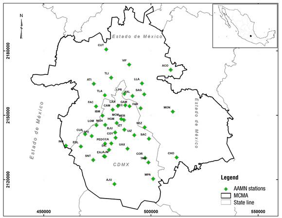
Figure 1. Study area and stations belonging to the Automatic Atmospheric Monitoring Network (AAMN) in Mexico City Metropolitan Area (MCMA).
The population living in the MCMA is 20.1 million, which represents 17 % of the national population, although slightly less than half live within Mexico City (INEGI, 2020). The dominant economic activities correspond to the service sector, commerce, and industrial activities (Espejel, 2019).
Pollutant database compilation and cleansing
Pollutant database, at station level, was downloaded from the Automatic Atmospheric Monitoring Network (AAMN) (https://datos.cdmx.gob.mx/dataset/red-automatica-de-monitoreo-atmosferico) for the period 1986-2021 for NOX, O3 and CO gases; 2000-2021 for PM10 and 2003-2021 for PM2.5. The AAMN database contains information on pollutant concentrations recorded at the hourly level at each monitoring station.
A total of 44 stations distributed in the MCMA were used; however, each pollutant had a different number of stations, since the sensors of some of them were not active on certain dates. Thus, 30, 35 and 31 stations were used for NOX, O3 and CO respectively, while 24 were used for PM2.5 and PM10.
The pollutant database provides information by date, time, and station. Therefore, to create a multi-annual database integrating all the stations, they were merged into a single file per pollutant using the R software. Subsequently, the data were transformed at day, month, and year levels for the corresponding analysis. The database was cleaned by removing null or erroneous data (<1 % of the total) that could affect the statistical parameters. Finally, the multi-year databases were exported in ‘shape’ format for further geostatistical analysis.
Descriptive statistical analysis
A descriptive statistical analysis (mean, median, minimum, and maximum) of pollutants NOX, CO, O3, PM2.5 and PM10 was performed; in addition, the correlation between them was evaluated using Spearman's coefficient, since the data were not adjusted to a normal distribution. The statistical analysis was performed in R version 4.0.5 (R Development Core Team, 2021).
Intra- and inter-annual variation of pollutants
Monthly average values per station and per zone were calculated to evaluate the temporal dynamics of pollutants over the course of the year. The temporal trend at the annual level was determined with the 'Theil-Sen' operator, a robust non-parametric method for obtaining temporal trends in short time series. The method fits a simple linear regression between all pairs of data and calculates the median of the slopes of all the lines (Akritas et al., 1995).
Spatial modeling methods and spatial interpolation
Spatial modeling is classified according to the following statistical techniques: a) spatial interpolation, b) spatial regression and c) Machine Learning (Chen et al., 2019; Perez et al., 2021). This study compared the predictive performance of four methods: 1) spatial interpolation (Universal Kriging) and 2) Machine Learning using supervised algorithms (Neural Network, Supported Vector Machine and Random Forest) (Castro et al., 2017; Pedrero et al., 2021). These methods were used to model the monthly and annual spatial distribution of each pollutant in the MCMA. The modeling and spatial interpolation analysis was carried out with the R software version 4.0.5 (R Development Core Team, 2021).
Interpolation with the Universal Kriging method was carried out with the ‘autoKrige’ function, which adjusts variograms in a grouped way from different models (spherical, exponential, and Gaussian), to finally perform the prediction with the optimal model in the areas with missing data (Estarlich et al., 2013).
For the Neural Network analysis, we used the statistical package 'R neuralnet', considering five layers of neurons arbitrarily chosen to train the model. For Supported Vector Machine, the 'ksvm' function of the 'kernlab' package was used, considering a polynomial Kernel algorithm with a penalty parameter of 25, which avoids overfitting the data (García & Lozano, 2007). Finally, Random Forest interpolation was carried out with the 'ranger' library in R, considering 1 000 trees and a single node (Espinosa-Zuñiga, 2020).
Unlike traditional interpolation methods (Universal Kriging), where the spatial location of the variables of interest (e.g., coordinates) is used, Maching Learning modeling and interpolation uses distance matrices between pairs of points, because coordinates are correlated with each other. Finally, with the average of all data, monthly and historical pollutant distribution maps were created.
Model validation and statistical performance
Model performance was evaluated using the coefficient of determination (R2), mean absolute error (MAE) and root mean square error (RMSE):
where,
y i = th observed value
n = number of predicted or observed values with i = 1, 2,…, n
These metrics help identifying the best model fitting the data; low RMSE values indicate a better fit, R2 indicates the goodness of fit of the model and MAE is a linear score and means that individual differences are weighted equally in the average (Beguin et al., 2017; Pérez et al., 2021).
Results and Discussion
Pollution historical statistics in the MCMA
The average of NOX was 20.8 ± 0.17 ppb with a historical maximum of 111 ppb (Hangares station, inactive) and a minimum of 0.1 ppb at Milpa Alta station (Table 1). Some authors indicate NOX decrease in the MCMA (Sandoval & Jaimes, 2002; Navarro, 2019), although the Secretariat of the Environment (SEDEMA) reports NOX increment in 2018. These authors emphasize that mobile sources contribute more than 85 % of pollutant emissions in the MCMA.
Table 1 Descriptive statistics of pollutants reported by the Automatic Atmospheric Monitoring Network (AAMN) in Mexico City Metropolitan Area.
| Pollutant | NOX (ppb) | CO (ppm) | O3 (ppb) | PM10 (µg∙m-3) | PM2.5 (µg∙m-3) |
|---|---|---|---|---|---|
| Average | 22.0 ± 0.17 | 1.86 ± 0.01 | 33.3 ± 0.12 | 47.7 ± 0.28 | 23.6 ± 0.14 |
| Median | 20.8 ± 0.17 | 1.35 ± 0.01 | 30.8 ± 0.12 | 44.4 ± 0.28 | 22.8 ± 0.14 |
| Minimum | 0.10(MPA) | 0.10(MPA) | 5.75(UIZ) | 11.40(INN) | 7.69(INN) |
| Maximum | 111.0(HAN*) | 13.0(TLA) | 96.9(CES*) | 145.0(XAL) | 68.2(SAG) |
| Period | 1986-2021 | 1986-2021 | 1986-2021 | 2000-2021 | 2003-2021 |
| n | 7 042 | 8 755 | 8 613 | 4 224 | 2 682 |
NOX: nitrogen oxides, CO: carbon monoxide, O3: ozone, PM10 and PM2.5: medium particulate matter or smaller than 10 and 2.5 µm, respectively. MPA: Milpa Alta, HAN: Hangares, TLA: Tlalnepantla, UIZ: UAM Iztapalapa, CES: Cerro de la Estrella, INN: Investigaciones Nucleares, XAL: Xalostoc, SAG: San Agustín, *Inactive stations.
The average CO was 1.86 ± 0.01 ppm, a value below the reference limit (9.0 ppm) of NOM-021-SSA1-202 (Secretaría de Salud, 2021). The maximum value was 13.0 ppm for Tlalpan station, and the minimum was 0.1 ppm for Milpa Alta station. SEDEMA mentions that CO was the pollutant with the highest total absolute emission in 2018 (646 434 Mg), representing 75.3 % of total air pollutant emissions, mainly product of incomplete combustion of gasoline, natural gas, oil, and other organic materials, according to that reported by Miller (2011).
O3 is a secondary gas formed by chemical and photochemical reactions between anthropogenic and natural primary emissions of precursors nitrogen oxides (NOX) and volatile organic compounds (VOC) or hydrocarbons (Calderón et al., 2000). O3 had a historical mean of 33.3 ± 0.12 ppb, with a maximum concentration of 96.9 ppb for the Cerro de la Estrella (CES) station, exceeding the limits established of 90.0 ppb by NOM-020-SSA1-2021 (Secretaría de Salud, 2021).
For PM10, an average of 47.7 ± 0.28 µg∙m-3 was obtained with a maximum of 145 µg∙m-3 for Xalostoc station, to the north of the MCMA. For this station, the main sources of suspended particulate matter are soil erosion, industries, and unpaved roads, which increase PM10 concentrations (Cervantes et al., 2005). The historical minimum of PM10 was 11.4 µg∙m-3 for Investigaciones Nucleares (INN) station, to the south of the MCMA. Meanwhile, PM2.5 particles have a historical mean of 23.6 ± 0.14 µg∙m-3 with a maximum for San Agustín (SAG) of 68.2 µg∙m-3 and a minimum of 7.69 µg∙m-3 for INN. Chow et al. (2002) mention that PM2.5 and PM10 particles are composed of nitrates, sulfates, ammonium, organic carbon, elemental carbon, and geological material, which in large quantities are harmful to the ecosystem.
Intra- and inter-annual variation of pollutants for MCMA
The highest NOX concentrations were recorded in December and January (>60 ppb) and decreased during June-August (<50 ppb) (Figure 2a). Some stations were also observed to exceed 100 ppb of NOX. These high concentrations are explained by the prevailing meteorological conditions and thermal inversions in winter, since low radiation and temperature, for example, are associated with high NOX concentrations (Sandoval & Jaimes, 2002).
CO had no significant variations over the year (Figure 2b), because concentrations of this compound depend on emissions from automobiles and industries, which remain constant over the course of the year (Madrigal et al., 2004). O3 (Figure 2c) the highest concentrations in April and May (>40 ppb), which coincides with the high level of solar radiation emitted in that period with different lengths of ultraviolet (UV) radiation (Wedyan et al., 2020). These, in turn, dissociate oxygen by photochemical reaction and, when available, react with other surrounding molecules (NOX, VOC and CO) allowing the formation of ozone. Possibly, cloudiness and lower radiation in December and January decrease UV radiation and, therefore, reduce O3 concentrations.
PM2.5 and PM10 depend on the emission of particulate matter from transportation, industry, residence, commerce, and services (Popovicheva et al., 2020). The period with the lowest concentration of these particles was during the rainy season (June-August, Figure 2d-e). This information is consistent with other studies indicating that PM concentrations decrease in the rainy season, which plays a role of wet removal of particles, but increase in dry periods due to accumulation of dust in foliage (Vinasco & Nastar, 2013; Zhou et al., 2020).
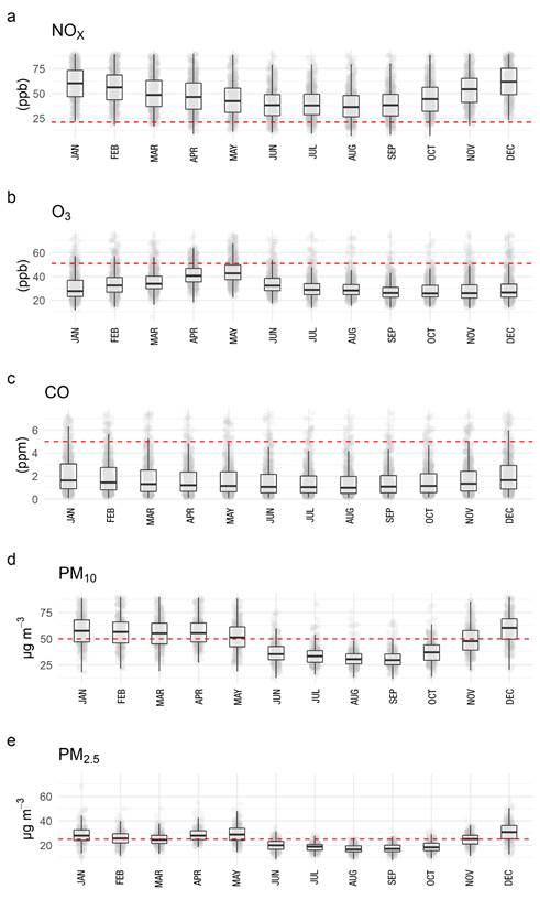
Figure 2 Monthly distribution of nitrogen oxides (NOX), ozone (O3), carbon monoxide (CO), particulate matter 10 (PM10) and 2.5 (PM2.5) in Mexico City Metropolitan Area. The dotted line indicates the permissible limit for pollutants according to NOM-023-SSA1-2021, NOM-020-SSA1-2021, NOM-021-SSA1-2021 and NOM-025-SSA1-2021.
Interannual variation of pollutants in the MCMA
Pollutant behavior at the interannual level was variable; for example, the maximum peak of NOX was recorded in 1993 (Figure 3), as well as O3 and CO. This coincides with studies that indicate that 1993 was the coldest year with the least precipitation in the MCMA (Pérez et al., 2010). These emissions exceeded the permissible pollution limits and the standards established for the central zone (Mercado et al., 1995). In that year, the highest pollution was caused by emissions from pharmaceutical companies, plastic articles and basic iron and steel industries, which emitted 64 % of atmospheric emissions in the Valley of Mexico. These companies use fossil fuels and increase CO, O3, NOX and VOC (Mercado et al., 1995). Since 1995, concentrations have decreased, particularly during the last decade, even though vehicle flow and number of vehicles have increased. This decrease can be attributed to improvements in automobile manufacturing, in addition to the implementation of the program to improve air quality in the Valley of Mexico (Sheinbaum, 2016).
The concentration of PM10 in the MCMA for the period 2000-2012 exceeded the limits of 50 µg∙m-3 indicated by NOM-025-SSA1-2021 (Secretaría de Salud, 2021). This increase is mainly attributed to emissions derived from transportation, industrial activity, and dust reincorporation from vehicle circulation (Villalobos, 2006). The lowest PM10 concentration was recorded in 2019 and 2020, which is probably related to the drastic closure of activities due to the COVID-19 pandemic. For example, in 2020, vehicular traffic was reduced in the MCMA, which restricted public mobility and reduced productive and industrial activities (Ale et al., 2020).
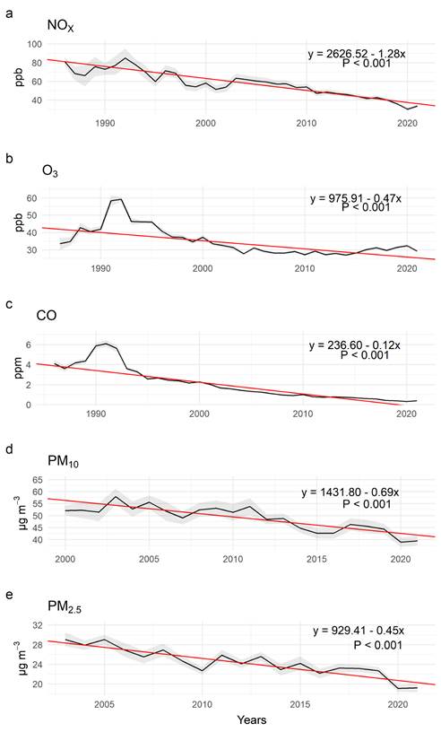
Figure 3 Interannual behavior of nitrogen oxides (NOX), ozone (O3), carbon monoxide (CO), particulate matter 10 µm (PM10) and 2.5 µm (PM2.5) in Mexico City Metropolitan Area. The light gray area represents the standard error among the stations included in the analysis.
PM2.5 exceeded the limit value established by NOM-025-SSA1-2021 and the World Health Organization (OMS, 2005: 25 µg∙m-3) in almost all the period analyzed; although in 2020, concentrations decreased, probably also because of the reduction of activities due to the social confinement derived from the COVID-19 pandemic. On the other hand, the temporal trends of NOX, CO, O3, PM10 and PM2.5 are negative and indicate a decrease of pollutants in MCMA (Figure 3). The pollutant with the highest decrement was NOX (-1.28 ppb∙yr-1) and the lowest was CO (-0.12 ppm∙yr-1), while PM2.5 and O3 had similar slopes -0.47 µg∙m-3∙yr-1 and -0.45 ppb∙yr-1, respectively.
On the other hand, Spearman's coefficient indicates a high correlation between NOX, CO, PM10 and PM2.5; however, O3 was not significantly associated with PM10 and PM2.5 (Table 2). The highest correlation values were between NOX, CO and O3, which could be attributed to the photochemical reaction involved in the formation of O3; that is, oxygen, once available, reacts with other NOX and CO compounds (Jenkin & Clemitshaw, 2000).
Table 2 Spearman correlation coefficient (***P < 0.001) among pollutants analyzed in Mexico City Metropolitan Area: nitrogen oxides (NOx), ozone (O3), carbon monoxide (CO), particulate matter 10 (PM10) and particulate matter 2.5 (PM2.5).
| Pollutant | NOX | O3 | CO | PM10 | PM2.5 |
|---|---|---|---|---|---|
| NOX | 1 | 0.95*** | 0.93*** | 0.85*** | 0.88*** |
| O3 | 1 | 0.77*** | 0.05 | -0.14 | |
| CO | 1 | 0.79*** | 0.86*** | ||
| PM10 | 1 | 0.86*** | |||
| PM2.5 | 1 |
Interpolation of pollutants in MCMA
No notable difference was found in the performance of the models Kriging Universal, Supported Vector Machine, Random Forest, and Neural Network at the monthly level; however, the Supported Vector Machine method was slightly superior with R2 values = 0.98; while the models with the lowest fit were Kriging Universal and Neural Network with R2 < 0.85.
Based on the historical average of each pollutant, the Supported Vector Machine model had the best goodness of fit with R2 greater than 0.95, except for CO, with R2 = 0.76 (Table 3). For MAE and RMSE, the models with the best fit were Neural Network and Supported Vector Machine. The Neural Network model had MAE and RMSE lower than 3.0, although R2 was lower than 0.8 for NOX, O3 and CO. Supported Vector Machine had MAE and RMSE lower than 3.0 for all pollutants except for NOX (MAE and RMSE between 4 and 6). On the other hand, the results indicated underestimation in the predicted values using Neural Network, Random Forest, and Universal Kriging, mainly for high values for the pollutants CO and O3 (Figure 4). Therefore, the Supported Vector Machine model had the best characteristics for modeling and interpolating the pollutants analyzed at the monthly level, as well as the historical average.
Table 3 Model validation statistics for the interpolation of historical averages by pollutant (NOX: nitrogen oxides, CO: carbon monoxide, O3: ozone, PM: particulate matter) in Mexico City Metropolitan Area.
| Method | Statistics | Pollutant | ||||
|---|---|---|---|---|---|---|
| NOX | O3 | CO | PM10 | PM2.5 | ||
| (ppb) | (ppb) | (ppm) | (µg∙m-3) | (µg∙m-3) | ||
| Neural Network | MAE | 1.52 | 0.49 | 0.07 | 1.05 | 0.35 |
| R2 | 0.79 | 0.64 | 0.37 | 0.98 | 0.94 | |
| RMSE | 1.58 | 2.76 | 0.07 | 1.08 | 0.36 | |
| Kriging Universal | MAE | 5.99 | 2.39 | 0.48 | 3.25 | 1.39 |
| R2 | 0.71 | 0.64 | 0.37 | 0.78 | 0.72 | |
| RMSE | 7.85 | 2.76 | 0.6 | 4.97 | 1.83 | |
| Random Forest | MAE | 5.43 | 2.57 | 0.42 | 0.86 | 0.55 |
| R2 | 0.86 | 0.81 | 0.69 | 0.8 | 0.83 | |
| RMSE | 6.72 | 2.85 | 0.54 | 1.18 | 0.86 | |
| Support Vector Machine | MAE | 4.3 | 1.65 | 0.28 | 3.27 | 1.05 |
| R2 | 0.98 | 0.98 | 0.76 | 0.99 | 0.98 | |
| RMSE | 5.59 | 1.96 | 0.34 | 4.74 | 1.44 | |
MAE: mean absolute error, RMSE: root mean square error.
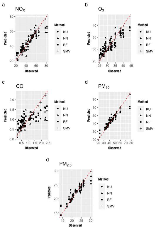
Figure 4 Observed vs. predicted values of data set by pollutants (NOX: nitrogen oxides, CO: carbon monoxide, O3: ozone, PM: particulate matter) using Kriging Universal (KU), Neural Network (NN), Random Forest (RF) and Support Vector Machine (SVM) in Mexico City Metropolitan Area. The dotted line indicates a 1:1 ratio.
Geostatistical modeling may have limitations in the selection of parameters, specially supervised Machine Learning methods. For example, Random Forest predictions can be expected to be beyond the range of observed values, if any data group presents confusion (Espinosa-Zuñiga, 2020). In the case of Neural Network, the main disadvantage is that neither its final equation nor the weights used in the model are known, making it a black box (Sheu, 2020). Kriging Universal requires an optimal variogram for the dataset to avoid extrapolations, and it is sensitive to a low number of points or a high variation between them (Shekaramiz et al., 2019). Finally, with Supported Vector Machine, Kernel and C parameters should be chosen appropriately, as they affect the complexity of the model (Cunha et al., 2022; Liu & Xu, 2014). Despite these limitations, Supported Vector Machine had the best fit for all pollutants and was therefore used to represent their spatial distribution.
Spatial dynamics of pollutants in MCMA
According to the spatial analysis, different patterns of pollutant distribution were found (Figure 5). For example, NOX showed a circular pattern, where the area with the highest concentration was located in the central zone of Mexico City with two stations with high values (La Merced and Xalostoc > 60 ppb). O3 had the highest concentrations at the Pedregal and Milpa Alta stations, located in the southern part of the study area. O3 concentration decreased towards the central and northern part of MCMA, indicating a high gradient in the southwestern quadrant. These results are consistent with the study by García (2009), who indicates that the highest pollutant areas are located downwind, away from emission sources, so high O3 concentration is located in mountainous areas south of Mexico City (Figure 5).
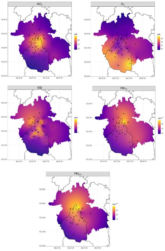
Figure 5 Spatial prediction of the average historical concentration of pollutants with the Machine Learning-Support Vector Machine method: nitrogen oxides (NOX, 1986-2021), ozone (O3, 1986-2021), carbon monoxide (CO, 1986-2021), particulate matter 10 µm (PM10, 2000-2021) and 2.5 µm (PM2.5, 2003-2021) in Mexico City Metropolitan Area. The black circles represent monitoring stations belonging to the Automatic Atmospheric Monitoring Network (AAMN).
The highest concentration of CO was found in the northwest central quadrant, probably due to a higher use of vehicles, which are the main source of emissions. However, some authors have reported a relationship between high CO concentrations and areas where the population has higher incomes in the Mexico Valley Metropolitan Area (MCMA), especially for CO and carbon dioxide emissions (CO2 eq) (Pérez et al., 2018).
PM10 and PM2.5 concentrations were higher in the center and decreased towards the west. The station with the highest concentration is Xalostoc with values above 70 µg∙m-3 of PM10 and 30 µg∙m-3 of PM2.5. This may be associated with the findings made by Cervantes et al. (2005), who affirm that the station is located in an area with evidence of soil erosion, presence of industries and unpaved roads.
Conclusions
The spatio-temporal dynamics varied among the pollutants analyzed. The highest NOX and CO concentrations were recorded from November to January, while O3 concentration decreased in that period and increased from April to May. The lowest particulate matter concentrations occurred from July to October and the highest in May. Regardless of the pollutant, concentrations decreased in recent years; NOX changes were most noticeable, and the lowest decrease was for CO. Key years such as 1993 or 2020 showed maximum peaks and troughs, mainly linked to the increase/closure of human activities. Although there were no notable differences among the interpolation methods, mainly among those belonging to the Machine Learning methods, the Support Vector Machine method had the best monthly and historical fit for all pollutants.


 texto en


