Introduction

Several studies have analyzed the effect of monetary policy in high-income economies without reaching a consensus. For example, in countries such as the United States, Australia and Sweden, expansionary monetary policy raises output (^{Corsetti and Müller,2015}; ^{Liu, 2021}; ^{Bhattarai et al., 2021}; ^{Ankargren and Shahnazarian, 2019}; ^{Inchauspe, 2021}). However, ^{Afonso and Gonçalves (2020)} argue that monetary policy is not effective in promoting economic growth in the US and the Eurozone; whilst ^{Bhattacharya and Jain (2020)}, analyze the effect of monetary policy on the food inflation rate in a set of developed and emerging economies, including Mexico, from 2006 to 2016 and their main finding is that unexpected contractionary monetary policy increases food inflation.

Regarding monetary policy reactions and its effects in the Mexican economy, ^{Loría and Ramirez (2008)} estimate a SVAR, identified through the New Keynesian model, using quarterly data ranging from 1985 to 2008, and they find that monetary policy instrument reacts to inflation as theory asserts (high inflation causes a contractive monetary policy, and vice versa) but does not respond to output fluctuations; however, according to their outcomes monetary policy does not affect inflation nor output.

^{Gaytán and Gonzalez (2008)} estimate a non-lineal VAR using monthly data from 1991 to 2005, their regressions indicate: a 2001 structural change in monetary policy transmission mechanism; monetary policy rate responding to real exchange rate, GDP, and inflation (also to expectations but only after 2001); as well, contractive monetary policy has the theoretical expected effects on output (after 2001), inflation and real exchange rate. Using the Generalized Method of Moments, ^{Cermeño and Villagómez (2012)} estimate a New Keynesian Open Economy Model for Mexican monthly data for the 1998-2008 period; evincing that interest rate reacts to output, inflation and exchange rate; also find output, inflation and exchange rate responding to interest rate. Finally, ^{Galindo and Guerrero (2003)} and ^{Loría and Ramirez (2011)} argue that Mexican Central Bank respond only to inflation rate variations, the formers also claim that interest rate affects inflation and output but not exchange rate.

Using Mexican data from January 2002 to August 2017, this paper estimates a SVAR recursively identified through a model that satisfies New Keynesian core assumptions. Two key contributions are 1) evince that expected inflation is formed according to static expectations hypothesis; 2) suggest nominal rigidities presence, which reinforces the reasons to assess the Mexican economy through the New Keynesian Model; moreover, impulse response functions indicate: expected inflation influencing observed inflation; interest rate endogenously reacting to output and inflation, as to expected inflation decreases; higher interest rate entailing lower inflation and output, and vice versa.

In the first section the theoretical model is exposed; next, estimation results are presented; and finally the conclusions are presented.

I. The Theoretical Model

The theoretical model that supports the empirical one (next section) is a New Keynesian Model simplified version. Several authors (^{Bofinger et al., 2006}, ^{Carlin and Soskice 2005}, ^{Chadha 2009}, ^{Mankiw 2010}, ^{Walsh 2002}) have proposed simpler versions that verify the Canonical Model (^{Clarida et al., 1999}) key assumptions, such as the producers are involved in monopolistic competition and set prices in the sense of ^{Calvo (1983)}; monetary policy instrument reacts to GDP and inflation; monetary policy is non-neutral as it affects aggregate demand components through ex-ante real interest rate, and this modifies output and price setting decisions. For example, ^{Bofinger et al., (2006)} introduce a static model with a credible Central Bank and prove that the monetary policy effects in GDP gap and inflation rate depend on the monetary policy rule it uses (with optimal or ad-hoc coefficients).

^{Mankiw (2010)} graphically exposes how the economy works using the dynamic IS function, the Phillips curve and an ad-hoc Taylor Rule, but, because assumes temporary exogenous shocks, it neglects to assess monetary policy reaction and its effects when trying to achieve GDP and inflation goals. ^{Walsh (2002)} uses a model with exogenous inflationary expectations and an ad-hoc reaction function that represents the trade-off among inflation and GDP faced by a Central Bank incapable to observe aggregate demand shocks, this feature and its transmission mechanism interpretation (as if expectations were endogenous) generated several critics (see ^{Bofinger et. al., 2006}). Therefore, in this section a Walsh model improved version with endogenous inflationary expectations and no ad-hoc reaction function (^{Lizarazu and Cernichiaro, 2016}) is exposed, and then, in next section, its empirical performance is assessed.

The model assumes a closed economy; static expectations, Etπt+1=πt; and an explicit inflation target πt*. The structural equations system includes a simplified IS curve (without expected income)

Where Yt is the difference among realized GDP and its potential level, this is the GDP gap; it is the nominal interest rate; Etπt+1 is expected inflation in t for t+1; rt- is the natural interest rate; ε1t is an aggregate demand shock; α is a positive parameter that represents aggregate income sensibility to real interest rate. The main feature of this equation is the negative relationship among ex-ante real interest rate and aggregate demand components, such as intertemporal consumption, investment and, in an open economy, net exports (^{Mankiw, 2010}).

The second structural equation is a Phillips Curve augmented by inflationary back-ward looking expectations¹

Where πt is inflation rate; and ε2t is an aggregate supply shock; ϕ is a positive parameter that represents inflation sensibility to GDP gap variations. The positive relationship among these variables is explained through the production positives effects on marginal costs, which motivates producers to reset higher prices in the same direction as the production level (^{Mankiw, 2010}).

The third equation is the economy reaction function

β is a positive parameter that represents Central Bank utility loss caused through GDP deviations. This equation is obtained after considering the optimal Central Bank behavior which equals the marginal losses and gains originated from GDP and inflation deviations from its actuals targets (^{Walsh, 2002}).

To close the model, it is necessary to specify the monetary policy rule in short run exogenous variables (structural shocks and expected inflation terms). In order to do it, the three equations presented must be solved to obtain the short run (before inflation expectations become endogenous and adjust to observed inflation) solutions for the endogenous variables Yt, πt, it Then, as is proved in ^{Lizarazu and Cernichiaro (2016)}, the (optimal) monetary policy rate can be expressed as an short run exogenous shocks function²

This equation means that interest rate will react to aggregate demand and supply shocks. It also indicates that the Central Bank will respond to expected inflation variations. We will evince how expectations adjusting to actual inflation, and the monetary policy rate reacting to it, are key for the economy to reach both inflation and output goals.

From equations (1) to (4) it can be noted that once the inflationary expectations adjust to observed inflation, and exogenous shocks become zero, in equilibrium the real interest rate will equal its natural level it-Et-1πt=rt-; the output gap will be zero; and inflation will coincide with the inflation goal as with expected inflation, πt=Etπt-1=πt.*.

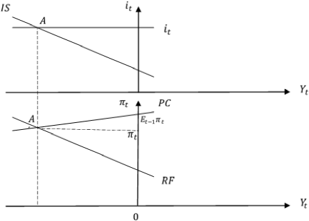
To better comprehend economy´s transmission mechanism, Figure 1 displays a scenario with both inflation and GDP below its respective targets. Figure 2 takes from such point and depicts inflation expectations adjust towards recently observed inflation, and interest rate changing in the same direction as expected inflation; these are the key steps for the economy to evolve until both inflation and GDP meet its targeted levels.

Source: Cernichiaro and ^{Lizarazu (2016)}.

Figure 1 Disequilibrium characterized by a negative output gap and low inflation 

Source: Cernichiaro and ^{Lizarazu (2016)}.

Figure 2 Equilibrium transition 

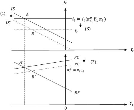
In Figure 1 output is below its potential level and inflation is lower than expected by households and producers.³ Then, diagram 2 displays how eventually inflationary expectation will diminish causing ex-ante real interest rate to rise, lowering current aggregate demand (The IS Curve shifts downwards); producers also adjust their expectations in the same direction (so the Phillips Curve, PC) shifts downwards too); Central Bank reacts lowering monetary policy rate trying to hinder aggregate´s demand contraction (Taylor Rule shifts downwards). As consequence, the economy goes from point A to B, this process will repeat until the economy reaches an equilibrium where real interest rate equals its natural level so output gap is equals zero, and observed inflation equals expected inflation and inflation target, πt=Etπt-1=πt.*.

In this section the theoretical model that supports next section´s structural vector autoregressive model (SVAR) was developed. Even if this is a simpler framework compared to the standard closed New Keynesian Model (^{Clarida et al., 1999}), it is useful to exhibit its main insights: a Central Bank that affects monopolistic competition producers’ output and price setting behavior through aggregate demand, thanks to monetary policy capability to modify ex-ante real interest rate.

As well, private sector´s inflationary expectations adjust to actual inflation and the Central Bank responding to it have been demonstrated to be fundamental for reaching output and inflation targets. The following section is aimed to assess three core propositions empirical performance: 1) Do Private´s Sector inflationary expectations are formed according to the static expectations hypothesis? 2) Does short run nominal interest rate actually react to inflationary expectations as New Keynesian theory asserts (higher expected inflation implies higher interest rate and vice versa)? 3) Does short run nominal interest rate affect GDP and inflation as New Keynesian theory asserts (higher interest rate implies lower GDP and lower inflation, and vice versa)?

II. The Empirical Model: SVAR

This section follows ^{Ouliaris et al., (2016)} exposition. Vector Autoregressive (VAR) models are linear multivariate time series models designed to capture the joint dynamic of those series; it treats each variable as endogenous and as a function of all variables lagged values,

Where G₀ is a nx1 vector of constants; G_j is a nxn coefficients matrix for J=1,…, p; e_t is a nx1 white noise innovations vector.

To reach an adequate VAR specification the residuals must satisfy Eeteτ'=0, if t≠τ, so an appropriate lags amount is required, if it is very small e_n,t may not be white noise residuals, nonetheless, if the number of lags is too big degrees of freedom will be lost, for each lag adds n2 coefficients to the regression. The VAR also must be covariance stationary, which implies that every variable in it is stationary. To verify this, two necessary conditions are required EXt=EXt+J=μ=μ1⋮μn, and E(Xt-μ)(Xt+J-μ)'=E(Xs-μ)(Xs+J-μ)'=ΓJ therefore, for a VAR to be stationary in covariance its first and second moments have to be finite and time invariant. The VARp process is stable if the np roots of the characteristic polynomial are inside the unitary circle,⁴ where the characteristic polynomial is the lag polynomial determinant det⁡[GL]=0, where GL is the polynomial of lags. If the VAR is stationary then it may be written as the infinite historical white noise shocks sum Xt=μ+∑i=0∞ψiet-i, where μ=G(L)-1G0; ψi matrix describes X_t time responses to each shocks sequence e_t .

Because this research aims to measure expected inflation response to observed inflation, monetary policy rate response to macroeconomic fluctuations, as its effects on GDP and inflation, the economy’s exogenous shocks must be isolated to distinguish why certain variable exhibit an specific time path, this means to recognize if its behavior is caused by endogenous contemporary correlations with other endogenous variables or if is generated by an structural shock. This is known as the structural vector autoregressive model identification.

Data, Estimation and Impulse-Reaction Functions

The variables included (GDP gap, expected inflation, inflation and short run nominal interest rate⁵) in the SVAR are the fundamental ones to assess the theoretical model empirical performance, which will be tested through the ensuing propositions: 1) recently observed inflation explains how expected inflation is formed; 2) short run nominal interest responds to output, inflation and expected inflation; 3) a short run nominal interest rise diminishes output and inflation. To do it, Mexican monthly data starting in January 2002 and ending in August 2017 is used.⁶ The sample starts in 2002 because that is when inflation targeting was implemented in Mexico (^{Ros, 2015}, and ends in August 2017 to avoid the negative outlier in output caused by the earthquake in Mexico in September 2017 (^{Banco de México, 2017: 4}).

The industrial activity index (retrieved from ^{Instituto Nacional de Estadistica y Geografía, INEGI}) approximates output, and its potential level is obtained through Hodrick-Prescott filter, output gap is the difference among them. Expected inflation is current month expectations for next month´s inflation (obtained from ^{Mexico´s Central Bank}), to obtain monthly expected inflation the mean of all surveyed observations was calculated. Inflation is first difference Consumer´s Price Index (INEGI) logarithm. Finally, also retrieved from ^{Mexico´s Central Bank}, 28 days Mexican Treasury Bonds (CETES for its Spanish meaning) is the short run nominal interest rate or monetary policy rate. Table 1 shows the descriptive statistics of these mentioned variables, and the Figure 3 displays their time series.

Table 1 Descriptive statistics of monetary policy rate, output gap, expected inflation and inflation, using monthly data from January 2002 to August 2017 

	Monetary policy rate	Output gap	Expected inflation	Observed inflation
Observations	188	187	188	187
Mean	5.6	9.90E-12	0.344	0.0033
Median	5.0	0.053	0.353	0.0037
Maximum	9.7	6.113	0.856	0.0168
Minimum	2.6	-7.048	-0.435	-0.0073
Standar deviaton	1.9	2.406	0.244	0.0035

Source: own elaboration with data from INEGI (Banco de Información Económica) and ^{Mexico´s Central Bank}(Política monetaria e inflación).

Source: own elaboration with data from INEGI (Banco de Información Económica) and ^{Mexico´s Central Bank}(Política monetaria e inflación).

Figure 3 Monetary policy rate, output gap, expected inflation and inflation, using monthly data from January 2002 to August 2017 

Therefore, the following SVAR contains 4 endogenous variables and a constants vector; it is recursively identified (^{Sims, 1992}) and its ordering is yt Etπt-1  πt  it. Hence, the identified matrix A is

A=1000a21100a31a3210a41a42a431

Where a21, a31,a32,a41,a42,a43 are the contemporary correlations among endogenous variables. Therefore, GDP gap only reacts contemporaneously to aggregate demand shocks; while monetary policy reacts contemporaneously to every exogenous shock, since is the last variable in the ordering.

Excluding monetary policy rate, every variable seems to be stationary (Table 2), nevertheless, only the overall stationarity of the VAR is necessary to guarantee the robustness of the findings and not the stationarity of the individual variables (^{Cuevas, 2009}; ^{Lütkepohl, 2006}).

The SVAR has 7 lags despite lag length selection criteria points out 12 lags, but this VAR is unstable (Tables 3 and 4). Therefore, the rule of thumb criteria⁷ is followed, the estimation continues with 7 lags and this model is stable (Table 5). Besides, as Figure 8 in Appendix 1 displays, correlogram does not indicate issues as short run autocorrelation, sinusoidal movement nor several high autocorrelations. Also the SVAR is serial correlation fee (Table 6)

Now it is possible to start answering the posed questions, first we asses if Mexican private sector inflationary expectations are formed according to the static expectations hypothesis. Figure 4 shows how inflationary expectations response to observed inflation.

Source: own estimations.

Figure 4 Expected inflation response to observed inflation 

The positive inflation shock (aggregate supply shock) is statistically significant until the third month, in this lapse expected inflation does note behaves as recently observed inflation. Nevertheless, expected inflation seems to follow quite close inflation fluctuations from the fourth month until year´s one end, when expected inflations stop being statistically significant. Therefore, evidence points that expected inflation does not react to inflation in the very short run (first three months), but it does from the fourth month until the rest of the year.

Now second question is appraised, even if the main interest is monetary policy rate´s reaction to expected inflation, it will be useful to see how it responds to output ad inflation too (Figure 5).

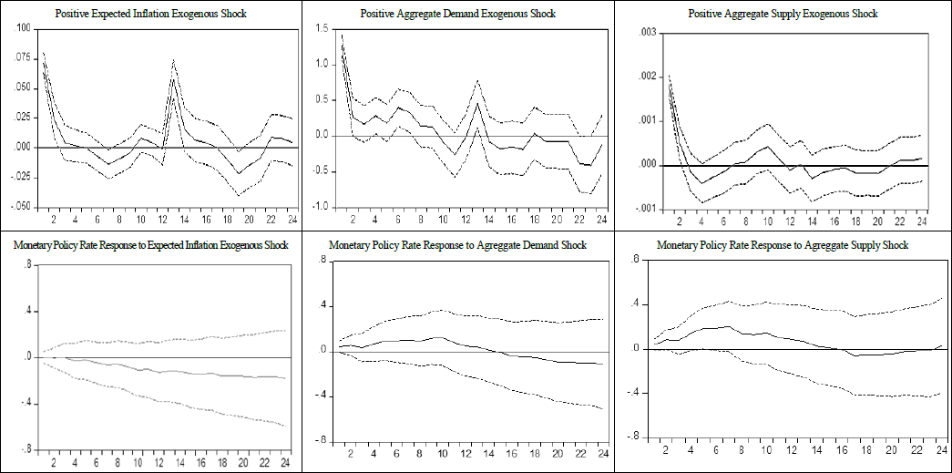
Source: own estimations.

Figure 5 Monetary policy rate response to expected inflation, output gap and observed inflation Response to Cholesky one Standard Deviations 

Positive aggregate demand shock is statistically significant for the first quarter, ^{Mexico´s Central Bank} answers increasing interest rate to contract aggregate demand, so producers diminish output which induce lower marginal costs and, hence, lower prices and inflation. Positive aggregate supply shock is statistically significant for the first three months, Central bank reacts increasing interest rate to lower inflation despite its contractive effects on output, after the shocks dilutes interest rate decreases. Expected inflation positive shock is statistically significant from the third to the 12^th month, interest rate does not seem to increase when expectations rise, however, when expectations start decreasing interest rate declines. As well, Figure 6 points out how actual inflation respond to expected inflation almost perfectly.

Source: own estimations.

Figure 6 Inflation response to expected inflation 

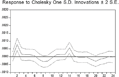
Finally, monetary policy effects on inflation and output is assessed (Figure 7).

Source: own estimations.

Figure 7 Monetary policy rate effects on observed inflation and output gap 

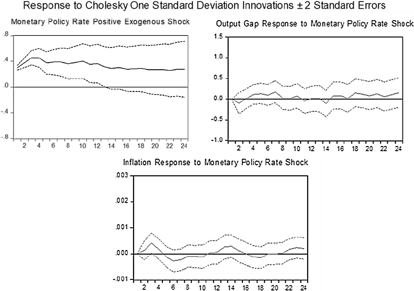
The positive monetary policy exogenous shock is statistically significant for 12 months, output decreases after nine months, which may be the time that takes to interest change to alter aggregate demand and producers to adjust output. In the other hand, inflation slightly decreases from the sixth month and onwards, as interest stabilizes it stops changing. Therefore, interest rate seems to affect both output and inflation, it takes producer almost three quarters to adjust production, while prices barely react, which suggests nominal rigidities (^{Galí 2008, 9}) presence for the Mexican economy, which reinforces the motifs to analyze it through the New Keynesian theory.

The New Keynesian Model seems to be doing empirically quite well for the Mexican case, inflationary expectations follow recent observed inflation; monetary policy rate responds to output gap, as to observed and expected inflation as well; finally, because its effects on inflation and output are the expected ones; therefore, it would make sense that the proposed transition to equilibrium verifies for the Mexican economy.

Conclusions

First, a synthetic New Keynesian model with static expectations and an optimal Taylor Rule was developed, whose main features are the Private Sector´s inflationary expectations adjust to recently observed inflation and Central´s Bank response to it, both features have been shown to be fundamental for reaching output and inflation targets. Using Mexico´s monthly data from January 2002 to August 2017, such theoretical framework was used to recursively identify a SVAR aimed to assess three of its core propositions empirical performance: 1) Private Sector´s inflationary expectations are formed according to the static expectations hypothesis. 2) Higher expected inflation observed inflation and GDP implies higher interest rate and vice versa. 3) Higher interest rate implies lower GDP and lower inflation, and vice versa.

Evidence points that expected inflation does not react to observed inflation in the very short run (first three months), but it does from the fourth month until the rest of the year. Also, interest rate does not seem to increase when expectations rise, however, when expectations start decreasing the Central Bank lowers interest rate. Is also shown that producers consider expected inflation when setting prices. Besides, when monetary policy rate rises, output decreases after seven months; and inflation decreases from the fifth month and stops changing when interest rate stabilizes; evidence also suggests nominal rigidities for the Mexican economy, which reinforces the motifs to analyze it through the New Keynesian theory.

The New Keynesian Model seems to do empirically quite well for the Mexican case, inflationary expectations follow recent observed inflation, monetary policy rate respond to output gap, inflation observed and expected as theory asserts; finally, because its effects on inflation and output are the expected ones, it would make sense that the proposed transition to equilibrium verifies for the Mexican economy. Nevertheless, it must be taking into account that even if the theoretical Canonical New Keynesian macroeconomic equations has the same form (except for its coefficients) for a closed and an open economy (^{Galí 2008, 165}), this analysis does not take into account any foreign factors that very well could contribute to explain better the Mexican (or other) economy; also other expectations hypothesis must be tested, such as rational expectations.

However, this research has two important limitations that can be addressed in the future. One is that it does not consider an open economy, adding variables such as real exchange rate and net exports, among others, could exhibit a better empirical performance. Some models that can be used for this task is the canonical New Keynesian model for an open economy by ^{Galí and Monacelli (2005)} or ^{Guerrieri et al., (2022)}, the latter also adds features to model the economic shocks caused by the Covid-19 pandemic. The other limitation is that this work lacks fiscal policy, whose complement with monetary policy alters the consequences on the business cycle and inflation (see (^{Corsetti and Müller, 2015}; ^{Liu, 2021}; ^{Bhattarai et al., 2021}; ^{Ankargren and Shahnazarian, 2019}; ^{Inchauspe, 2021}).